## Chart: Gibbs Error and Generalization Error vs. Steps/Updates
### Overview
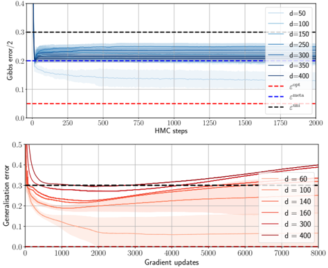
The image presents two line charts comparing Gibbs error and generalization error against the number of HMC steps and gradient updates, respectively. The charts illustrate the performance of different models (parameterized by 'd') during training. The top chart shows Gibbs error/2 versus HMC steps, while the bottom chart shows generalization error versus gradient updates.
### Components/Axes
**Top Chart:**
* **Title:** Gibbs error/2
* **X-axis:** HMC steps (range: 0 to 2000)
* **Y-axis:** Gibbs error/2 (range: 0 to 0.4)
* **Data Series (d values):** 50, 100, 150, 250, 300, 350, 400
* **Horizontal Lines:**
* Red dashed line: labeled as "e^opt" at approximately 0.05
* Blue dashed line: labeled as "e^meta" at approximately 0.22
* Black dashed line: labeled as "e^uni" at approximately 0.30
**Bottom Chart:**
* **Title:** Generalisation error
* **X-axis:** Gradient updates (range: 0 to 8000)
* **Y-axis:** Generalisation error (range: 0 to 0.5)
* **Data Series (d values):** 60, 100, 140, 160, 300, 400
* **Horizontal Lines:**
* Black dashed line: labeled as "e^uni" at approximately 0.30
### Detailed Analysis
**Top Chart (Gibbs error/2 vs. HMC steps):**
* **d = 50 (lightest blue):** Starts at approximately 0.4, rapidly decreases to approximately 0.2, and then plateaus.
* **d = 100 (lighter blue):** Starts at approximately 0.35, decreases to approximately 0.22, and then plateaus.
* **d = 150 (mid-light blue):** Starts at approximately 0.3, decreases to approximately 0.23, and then plateaus.
* **d = 250 (mid-blue):** Starts at approximately 0.27, decreases to approximately 0.23, and then plateaus.
* **d = 300 (darker blue):** Starts at approximately 0.25, decreases to approximately 0.23, and then plateaus.
* **d = 350 (dark blue):** Starts at approximately 0.24, decreases to approximately 0.23, and then plateaus.
* **d = 400 (darkest blue):** Starts at approximately 0.23, remains relatively constant around 0.23.
**Bottom Chart (Generalisation error vs. Gradient updates):**
* **d = 60 (lightest red):** Starts at approximately 0.5, decreases to approximately 0.25 around 1000 gradient updates, and then gradually increases to approximately 0.38.
* **d = 100 (lighter red):** Starts at approximately 0.45, decreases to approximately 0.25 around 1000 gradient updates, and then gradually increases to approximately 0.35.
* **d = 140 (mid-light red):** Starts at approximately 0.4, decreases to approximately 0.25 around 1000 gradient updates, and then gradually increases to approximately 0.33.
* **d = 160 (mid-red):** Starts at approximately 0.38, decreases to approximately 0.26 around 1000 gradient updates, and then gradually increases to approximately 0.32.
* **d = 300 (darker red):** Starts at approximately 0.35, decreases to approximately 0.27 around 1000 gradient updates, and then gradually increases to approximately 0.31.
* **d = 400 (darkest red):** Starts at approximately 0.33, decreases to approximately 0.28 around 1000 gradient updates, and then gradually increases to approximately 0.30.
### Key Observations
* In the top chart, all Gibbs error lines converge to a similar value after a certain number of HMC steps.
* In the bottom chart, all generalization error lines initially decrease and then increase, suggesting an initial learning phase followed by overfitting.
* The "e^opt" line represents the optimal error, "e^meta" represents the meta error, and "e^uni" represents the uniform error.
### Interpretation
The charts demonstrate the relationship between model complexity (represented by 'd'), training steps/updates, and error rates. The top chart suggests that Gibbs error converges relatively quickly with HMC steps, regardless of the model complexity. The bottom chart indicates that generalization error initially decreases as the models learn, but then increases as the models start to overfit the training data. The optimal error (e^opt) is significantly lower than the meta error (e^meta) and uniform error (e^uni), suggesting that the models can achieve better performance with proper training and regularization techniques. The uniform error (e^uni) serves as a baseline, and the models generally perform better than this baseline after sufficient training.