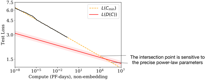
\n ## Chart: Test Loss vs. Compute (PF-days) ### Overview The image presents a line chart comparing two loss functions, L(Cmin) and L(D(C)), against the compute cost measured in PF-days (non-embedding). The chart aims to illustrate the relationship between computational effort and test loss for two different approaches. Shaded regions around each line indicate uncertainty or variance. ### Components/Axes * **X-axis:** "Compute (PF-days), non-embedding" - Logarithmic scale from 10^-8 to 10^7. * **Y-axis:** "Test Loss" - Linear scale from 1.5 to 7.5. * **Legend:** Located in the top-right corner. * `L(Cmin)` - Represented by a dashed orange line. * `L(D(C))` - Represented by a solid red line. * **Annotation:** Located on the right side of the chart: "The intersection point is sensitive to the precise power-law parameters". ### Detailed Analysis **L(Cmin) - Dashed Orange Line:** The orange line starts at approximately 7.0 at 10^-8 compute and slopes downward, becoming relatively flat around 10^2 compute. * At 10^-8 compute: Test Loss ≈ 7.0 * At 10^-5 compute: Test Loss ≈ 5.0 * At 10^-2 compute: Test Loss ≈ 3.0 * At 10^0 compute: Test Loss ≈ 2.0 * At 10^4 compute: Test Loss ≈ 1.6 * At 10^7 compute: Test Loss ≈ 1.5 **L(D(C)) - Solid Red Line:** The red line begins at approximately 6.0 at 10^-8 compute and exhibits a steeper downward slope than the orange line. It intersects with the orange line around 10^2 compute. * At 10^-8 compute: Test Loss ≈ 6.0 * At 10^-5 compute: Test Loss ≈ 4.0 * At 10^-2 compute: Test Loss ≈ 2.0 * At 10^0 compute: Test Loss ≈ 1.7 * At 10^4 compute: Test Loss ≈ 1.3 * At 10^7 compute: Test Loss ≈ 1.2 **Shaded Regions:** Both lines are surrounded by shaded regions, indicating uncertainty. The shaded regions are wider at lower compute values and become narrower as compute increases. This suggests greater uncertainty in the loss values at lower compute levels. ### Key Observations * The red line (L(D(C))) consistently shows lower test loss values compared to the orange line (L(Cmin)) across the entire range of compute values. * The intersection point of the two lines is around 10^2 compute, where the test loss is approximately 2.0. * The annotation highlights the sensitivity of this intersection point to the specific power-law parameters used in the model. * The uncertainty (represented by the shaded regions) is higher at lower compute values, indicating less confidence in the loss estimates in that region. ### Interpretation The chart suggests that the approach represented by L(D(C)) generally achieves lower test loss for a given compute cost compared to L(Cmin). However, the optimal choice between the two approaches depends on the specific compute budget and the sensitivity of the intersection point to the power-law parameters. The intersection point represents a potential trade-off point where the benefits of L(D(C)) may no longer outweigh the additional computational cost. The higher uncertainty at lower compute values suggests that more data or analysis may be needed to accurately assess the performance of both approaches in that region. The annotation implies that the precise shape of the curves, and therefore the intersection point, is dependent on the underlying model parameters, and careful calibration is required.