## Diagram: Reservoir Computing System Performance
### Overview
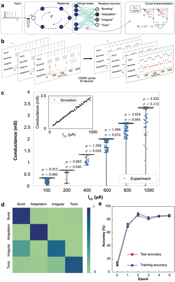
The image presents a multi-panel diagram illustrating a reservoir computing system, its implementation, and performance characteristics. Panel (a) shows a schematic of the reservoir computing architecture. Panel (b) displays raster plots of neuron activity for different neuron types. Panel (c) presents a scatter plot comparing simulated and experimental conductance data. Panel (d) shows a heatmap of neuron type distribution and a graph of training/testing accuracy over epochs.
### Components/Axes
**Panel a:**
* **Labels:** Input, Reservoir, Virtual nodes, Readout neurons, Circuit implementation, Icc Control, G*, G.
* **Diagram Elements:** Input signal flowing into a reservoir of interconnected neurons, readout layer connecting the reservoir to output neurons, and a circuit implementation showing transistors.
* **Annotations:** τ (time constant), W<sub>ij</sub> (weights).
**Panel b:**
* **Labels:** Bursting, Adaptation, Irregular, Tonic, Time (ms).
* **Axes:** X-axis: Time (0-1000 ms). Y-axis: Neuron index (25 devices).
* **Legend:** Bursting (orange), Adaptation (purple), Irregular (blue), Tonic (green).
**Panel c:**
* **Labels:** Conductance (mS), I<sub>cc</sub> (µA), Simulation, Experiment.
* **Axes:** X-axis: I<sub>cc</sub> (µA) (0-1100). Y-axis: Conductance (mS) (0-4).
* **Annotations:** μ (mean), σ (standard deviation) values for simulation and experiment.
* **Inset:** A smaller scatter plot showing simulation data.
**Panel d:**
* **Labels:** Burst, Adaptation, Irregular, Tonic, Epoch.
* **Heatmap Axes:** X-axis: Neuron type (Burst, Adaptation, Irregular, Tonic). Y-axis: Neuron type (Burst, Adaptation, Irregular, Tonic).
* **Accuracy Graph Axes:** X-axis: Epoch (1-5). Y-axis: Accuracy (%) (0-100).
* **Legend:** Test accuracy (black), Training accuracy (red).
### Detailed Analysis or Content Details
**Panel a:**
The diagram illustrates a reservoir computing system. An input signal is fed into a reservoir of randomly connected neurons. The reservoir's state is then mapped to output neurons via a readout layer. The circuit implementation shows a transistor-based circuit with Icc control and gate voltages G* and G.
**Panel b:**
Raster plots show the spiking activity of different neuron types over time. The plots display 25 devices.
* **Bursting:** Shows sporadic, high-frequency bursts of activity.
* **Adaptation:** Shows activity that adapts over time, decreasing in frequency.
* **Irregular:** Shows a relatively constant, random spiking pattern.
* **Tonic:** Shows a consistent, low-frequency spiking pattern.
**Panel c:**
A scatter plot compares simulated and experimental conductance data as a function of I<sub>cc</sub>.
* **Simulation:** The simulation data shows a positive correlation between conductance and I<sub>cc</sub>. The mean (μ) is approximately 0.312 mS, with a standard deviation (σ) of approximately 0.060 mS.
* **Experiment:** The experimental data also shows a positive correlation, but with a wider spread. The mean (μ) is approximately 1.330 mS, with a standard deviation (σ) of approximately 0.033 mS.
* **Inset:** The inset shows a zoomed-in view of the simulation data, revealing a more detailed relationship between conductance and I<sub>cc</sub>.
* **Overall:** The experimental data has a higher conductance range than the simulation data. The mean (μ) for the experiment is approximately 2.658 mS, with a standard deviation (σ) of approximately 0.084 mS. The mean (μ) for the experiment is approximately 3.325 mS, with a standard deviation (σ) of approximately 0.112 mS.
**Panel d:**
* **Heatmap:** The heatmap shows the distribution of neuron types. The diagonal elements (Burst-Burst, Adaptation-Adaptation, etc.) are the most prominent, indicating a higher proportion of neurons of the same type.
* **Accuracy Graph:** The graph shows the training and testing accuracy of the reservoir computing system over epochs.
* **Training Accuracy:** Starts at approximately 20% at epoch 1 and increases to approximately 80% by epoch 5.
* **Test Accuracy:** Starts at approximately 40% at epoch 1 and plateaus at approximately 70% by epoch 3, remaining relatively stable through epoch 5.
### Key Observations
* The experimental conductance values are significantly higher than the simulated values.
* The accuracy graph shows a clear overfitting trend, with training accuracy increasing while test accuracy plateaus.
* The heatmap suggests a preference for neurons of the same type within the reservoir.
* The raster plots in panel (b) clearly differentiate the spiking behavior of the four neuron types.
### Interpretation
The diagram demonstrates the implementation and performance of a reservoir computing system. The comparison between simulation and experiment highlights the discrepancies between theoretical models and real-world implementations, potentially due to factors not captured in the simulation. The accuracy graph reveals a potential overfitting issue, suggesting that the model is memorizing the training data rather than generalizing to unseen data. The heatmap provides insight into the composition of the reservoir, indicating a non-uniform distribution of neuron types. The different spiking patterns observed in the raster plots suggest that the neuron types contribute differently to the reservoir's dynamics. The overall system demonstrates the potential of reservoir computing for complex information processing, but also highlights the challenges of bridging the gap between simulation and experiment and avoiding overfitting. The Icc control and transistor-based circuit implementation in panel (a) suggest a physical realization of the reservoir computing concept. The data suggests that the system is capable of learning, but requires careful tuning to avoid overfitting and achieve optimal performance.