## Diagram: Neural Network Architecture and Magnetic Properties
### Overview
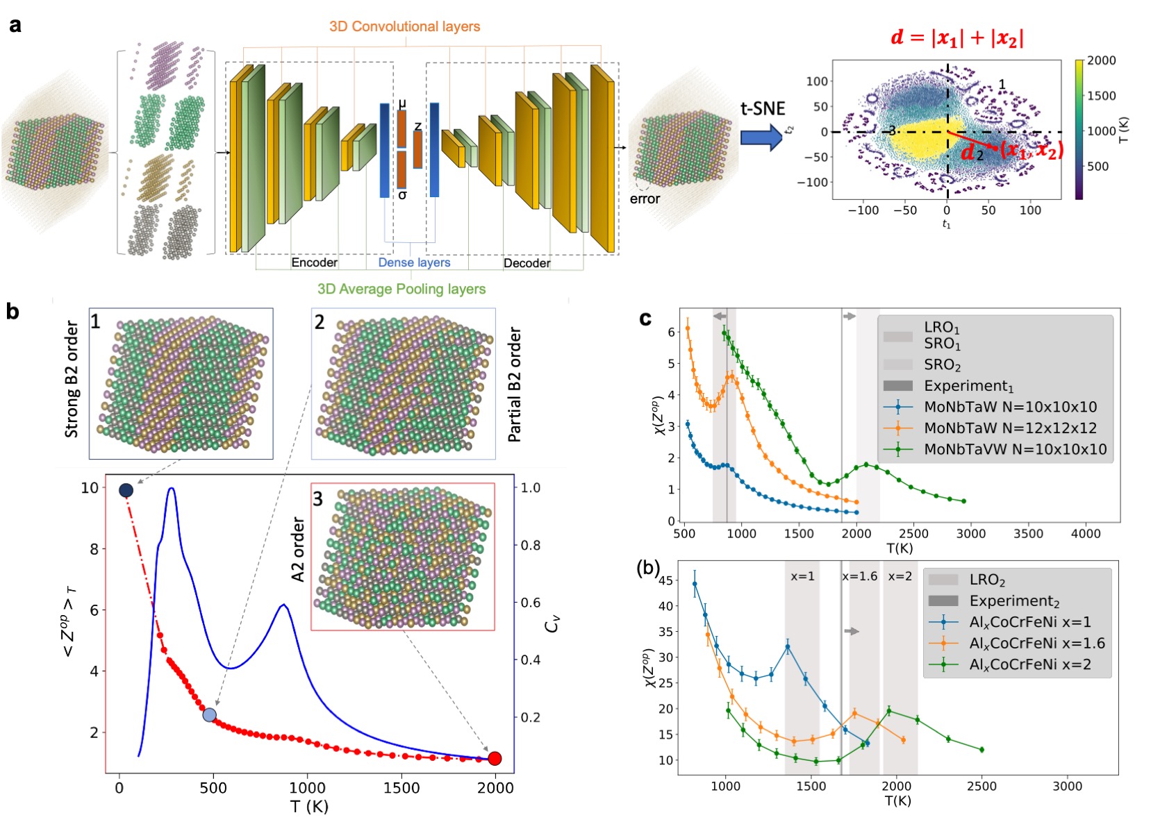
The image presents a multi-panel diagram illustrating a neural network architecture used to analyze magnetic properties of materials. Panel (a) depicts the neural network structure. Panel (b) shows visualizations of different magnetic orderings and their corresponding temperature dependence. Panel (c) and (b) display plots of X(Z<sub>op</sub>) versus temperature (T) for different materials and compositions.
### Components/Axes
**Panel (a): Neural Network**
* **Title:** "a"
* **Components:** 3D Convolutional layers, Encoder, Dense layers, Decoder, Error.
* **Diagram:** Shows a flow from input (3D Convolutional layers) through an Encoder and Dense layers, then a Decoder, resulting in an error signal.
* **Equation:** d = |x<sub>1</sub>| + |x<sub>2</sub>|
* **t-SNE Plot:** X-axis labeled "t<sub>1</sub>", Y-axis labeled "t<sub>2</sub>", Color bar ranging from approximately 500 to 2000. Points are colored based on the colorbar. Points are clustered into three groups labeled 1, 2, and 3.
**Panel (b): Magnetic Orderings & Temperature Dependence**
* **Title:** "b"
* **Sub-panels:** Two visualizations of atomic arrangements representing "Strong B2 order" (1) and "Partial B2 order" (2). Below these, a plot of <Z<sub>op</sub>> vs. T.
* **Plot Axes:** X-axis labeled "T (K)", Y-axis labeled "<Z<sub>op</sub>>".
* **Curves:** Two curves are plotted: a blue curve representing "A2 order" and a purple curve representing "B2 order".
* **Colorbar:** Ranges from approximately 0.0 to 1.0, representing a value labeled "ζ".
**Panel (c): X(Z<sub>op</sub>) vs. T for Different Materials**
* **Title:** "c"
* **Axes:** X-axis labeled "T(K)", Y-axis labeled "X(Z<sub>op</sub>)".
* **Data Series:**
* "Experiment" (Black dashed line)
* "MoNbTaW N=10x10x10" (Red line)
* "MoNbTaW N=12x12x12" (Green line)
* "MoNbTaW N=10x10x10" (Blue line)
**Panel (b): X(Z<sub>op</sub>) vs. T for Different Compositions**
* **Title:** "(b)"
* **Axes:** X-axis labeled "T(K)", Y-axis labeled "X(Z<sub>op</sub>)".
* **Data Series:**
* "Experiment<sub>2</sub>" (Black dashed line)
* "Al<sub>x</sub>CoCrFeNi x=1" (Red line)
* "Al<sub>x</sub>CoCrFeNi x=1.6" (Green line)
* "Al<sub>x</sub>CoCrFeNi x=2" (Blue line)
* **Labels:** x=1, x=1.6, x=2 are indicated near the corresponding lines.
### Detailed Analysis or Content Details
**Panel (a):** The t-SNE plot shows three distinct clusters of points. Cluster 1 (red) is centered around (approximately 50, 50) and has values ranging from 500 to 2000. Cluster 2 (blue) is centered around (-50, -50) and has values ranging from 500 to 2000. Cluster 3 (purple) is more dispersed.
**Panel (b):** The <Z<sub>op</sub>> vs. T plot shows a sharp decrease in <Z<sub>op</sub>> from approximately 8 to 0 around 500K, corresponding to the transition from B2 order to A2 order. The B2 order curve (purple) remains relatively high until around 500K, then drops rapidly. The A2 order curve (blue) remains low throughout the temperature range. The colorbar indicates that ζ is high for strong B2 order and low for partial B2 order.
**Panel (c):** The X(Z<sub>op</sub>) vs. T plot shows that the experimental data (black dashed line) initially increases, reaches a maximum around 1000K, and then decreases. The MoNbTaW simulations with different sizes (red, green, blue) generally follow the experimental trend, but with varying magnitudes. The N=10x10x10 simulation (red) closely matches the experimental data up to approximately 2000K.
**Panel (b):** The X(Z<sub>op</sub>) vs. T plot shows that the experimental data (black dashed line) initially increases, reaches a maximum around 1000K, and then decreases. The Al<sub>x</sub>CoCrFeNi simulations with different compositions (red, green, blue) generally follow the experimental trend, but with varying magnitudes. The x=1 simulation (red) closely matches the experimental data up to approximately 2000K.
### Key Observations
* The neural network architecture in panel (a) suggests a dimensionality reduction technique (Encoder) followed by reconstruction (Decoder).
* The t-SNE plot in panel (a) indicates that the neural network can effectively separate data into three distinct classes.
* The temperature dependence of <Z<sub>op</sub>> in panel (b) reveals a phase transition from B2 to A2 order.
* The simulations in panel (c) and (b) generally agree with the experimental data, suggesting the validity of the model.
* The size of the simulation cell (N) in panel (c) affects the accuracy of the results.
* The composition (x) of the Al<sub>x</sub>CoCrFeNi alloy in panel (b) affects the accuracy of the results.
### Interpretation
The diagram demonstrates the use of a neural network to analyze the magnetic properties of materials. The neural network is trained to identify different magnetic orderings (B2, A2) and predict their temperature dependence. The t-SNE plot suggests that the neural network can effectively learn to distinguish between these orderings. The simulations in panels (c) and (b) show that the model can accurately reproduce the experimental results, providing insights into the underlying physics of these materials. The discrepancies between the simulations and the experimental data may be due to the limitations of the model or the experimental setup. The varying results based on simulation cell size and alloy composition suggest that these parameters are important for accurate modeling. The overall goal appears to be to use machine learning to accelerate the discovery and design of new magnetic materials.