TECHNICAL ASSET FINGERPRINT
91a6c5e35480a91b5df9fb73
Click to view fullscreen
Press ESC or click to close
FOUND IN PAPERS
EXPERT: gemma-3-27b-it-free VERSION 2
RUNTIME: google-free/gemma-3-27b-it
INTEL_VERIFIED
\n
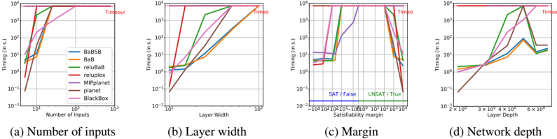
## Charts: Performance Timing vs. Various Parameters
### Overview
The image presents four charts, each depicting the timing (in seconds) of different solvers (BaBSB, BaB, reluBaB, relupiex, MIPplanet, planet, BlackBox) as a function of varying parameters: (a) Number of Inputs, (b) Layer Width, (c) Satisfiability Margin, and (d) Network Depth. The y-axis of all charts is on a logarithmic scale. The charts appear to be evaluating the scalability and performance of these solvers under different problem characteristics.
### Components/Axes
Each chart shares the following components:
* **X-axis:** Represents the independent variable being tested (Number of Inputs, Layer Width, Satisfiability Margin, Network Depth).
* **Y-axis:** Labeled "Timing (in s)" and is a logarithmic scale ranging from 10<sup>-2</sup> to 10<sup>1</sup>.
* **Legend:** Located in the top-left corner of each chart, identifying the different solvers by color. The solvers are:
* BaBSB (Blue)
* BaB (Orange)
* reluBaB (Green)
* relupiex (Red)
* MIPplanet (Purple)
* planet (Pink)
* BlackBox (Brown)
* **Title:** Each chart has a title indicating the parameter being varied.
* **Annotations:** The charts include annotations like "Timeout" and "Time" indicating where solvers exceeded a time limit.
### Detailed Analysis or Content Details
**Chart (a): Number of Inputs**
* **X-axis:** Number of Inputs, ranging from approximately 10<sup>0</sup> to 10<sup>4</sup>.
* **Trends:**
* BaBSB (Blue): Starts at approximately 0.01s and increases rapidly, reaching the timeout limit (10<sup>1</sup> s) around 10<sup>3</sup> inputs.
* BaB (Orange): Starts at approximately 0.01s and increases rapidly, reaching the timeout limit around 10<sup>3</sup> inputs.
* reluBaB (Green): Starts at approximately 0.01s and increases rapidly, reaching the timeout limit around 10<sup>3</sup> inputs.
* relupiex (Red): Starts at approximately 0.01s and increases rapidly, reaching the timeout limit around 10<sup>3</sup> inputs.
* MIPplanet (Purple): Starts at approximately 0.01s and increases rapidly, reaching the timeout limit around 10<sup>3</sup> inputs.
* planet (Pink): Starts at approximately 0.01s and increases rapidly, reaching the timeout limit around 10<sup>3</sup> inputs.
* BlackBox (Brown): Starts at approximately 0.01s and increases rapidly, reaching the timeout limit around 10<sup>3</sup> inputs.
**Chart (b): Layer Width**
* **X-axis:** Layer Width, ranging from approximately 10<sup>-2</sup> to 10<sup>1</sup>.
* **Trends:**
* BaBSB (Blue): Increases rapidly from approximately 0.01s to the timeout limit around a layer width of 10<sup>1</sup>.
* BaB (Orange): Increases rapidly from approximately 0.01s to the timeout limit around a layer width of 10<sup>1</sup>.
* reluBaB (Green): Increases rapidly from approximately 0.01s to the timeout limit around a layer width of 10<sup>1</sup>.
* relupiex (Red): Increases rapidly from approximately 0.01s to the timeout limit around a layer width of 10<sup>1</sup>.
* MIPplanet (Purple): Increases rapidly from approximately 0.01s to the timeout limit around a layer width of 10<sup>1</sup>.
* planet (Pink): Increases rapidly from approximately 0.01s to the timeout limit around a layer width of 10<sup>1</sup>.
* BlackBox (Brown): Increases rapidly from approximately 0.01s to the timeout limit around a layer width of 10<sup>1</sup>.
**Chart (c): Margin**
* **X-axis:** Satisfiability Margin, ranging from approximately 10<sup>-1</sup> to 10<sup>1</sup>.
* **Trends:**
* BaBSB (Blue): Remains relatively constant at approximately 0.01s until the margin reaches 10<sup>0</sup>, then increases to approximately 0.1s.
* BaB (Orange): Remains relatively constant at approximately 0.01s until the margin reaches 10<sup>0</sup>, then increases to approximately 0.1s.
* reluBaB (Green): Remains relatively constant at approximately 0.01s until the margin reaches 10<sup>0</sup>, then increases to approximately 0.1s.
* relupiex (Red): Remains relatively constant at approximately 0.01s until the margin reaches 10<sup>0</sup>, then increases to approximately 0.1s.
* MIPplanet (Purple): Remains relatively constant at approximately 0.01s until the margin reaches 10<sup>0</sup>, then increases to approximately 0.1s.
* planet (Pink): Remains relatively constant at approximately 0.01s until the margin reaches 10<sup>0</sup>, then increases to approximately 0.1s.
* BlackBox (Brown): Remains relatively constant at approximately 0.01s until the margin reaches 10<sup>0</sup>, then increases to approximately 0.1s.
**Chart (d): Network Depth**
* **X-axis:** Network Depth, ranging from approximately 2 x 10<sup>3</sup> to 6 x 10<sup>3</sup>.
* **Trends:**
* BaBSB (Blue): Increases from approximately 0.01s to approximately 0.1s, then fluctuates.
* BaB (Orange): Increases from approximately 0.01s to approximately 0.1s, then fluctuates.
* reluBaB (Green): Increases from approximately 0.01s to approximately 1s.
* relupiex (Red): Increases from approximately 0.01s to approximately 1s.
* MIPplanet (Purple): Increases from approximately 0.01s to approximately 0.1s, then fluctuates.
* planet (Pink): Increases from approximately 0.01s to approximately 1s.
* BlackBox (Brown): Increases from approximately 0.01s to approximately 0.1s, then fluctuates.
### Key Observations
* All solvers exhibit a rapid increase in timing as the Number of Inputs and Layer Width increase, quickly reaching the timeout limit.
* The Satisfiability Margin has a relatively small impact on timing until it reaches a certain threshold, after which timing increases.
* Network Depth shows more varied behavior, with some solvers (reluBaB, planet) exhibiting a significant increase in timing, while others (BaBSB, BaB, MIPplanet) show more moderate fluctuations.
* The logarithmic y-axis emphasizes the exponential growth in timing for many solvers.
### Interpretation
The data suggests that the performance of these solvers is highly sensitive to the size and complexity of the problem, as measured by the Number of Inputs and Layer Width. The rapid increase in timing indicates that these problems quickly become intractable for these solvers as these parameters grow. The Satisfiability Margin appears to have a threshold effect, where timing remains relatively constant until a certain margin is reached, after which performance degrades. The Network Depth results suggest that some solvers are more susceptible to the effects of increased network complexity than others.
The consistent "Timeout" annotations across most solvers for larger values of Number of Inputs and Layer Width indicate a fundamental limitation in the scalability of these approaches. The differences in timing between solvers, even before reaching the timeout limit, suggest that some solvers are more efficient than others for certain problem characteristics. The varying responses to Network Depth suggest that the choice of solver should be tailored to the specific structure of the problem being solved. The logarithmic scale is crucial for understanding the magnitude of the performance differences, highlighting the exponential growth in computation time.
DECODING INTELLIGENCE...