TECHNICAL ASSET FINGERPRINT
9289ad79aeeb263217109216
Click to view fullscreen
Press ESC or click to close
FOUND IN PAPERS
EXPERT: healer-alpha-free VERSION 1
RUNTIME: free/openrouter/healer-alpha
INTEL_VERIFIED
## Normalized MSE vs Time (Equations Discovered on Noisy Data): Multi-Chart Analysis
### Overview
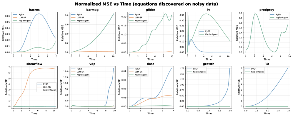
The image is a composite figure containing ten individual line charts arranged in a 2x5 grid. The overarching title is "Normalized MSE vs Time (equations discovered on noisy data)". Each subplot displays the performance of up to three different symbolic regression methods over time, measured by "Relative MSE" (Mean Squared Error). The charts compare the methods' ability to discover equations from noisy data across ten different dynamical systems or datasets.
### Components/Axes
* **Main Title:** "Normalized MSE vs Time (equations discovered on noisy data)" - centered at the top.
* **Subplot Titles:** Each of the ten charts has a title corresponding to a specific system/dataset: `bacres`, `barmag`, `glider`, `lv`, `predprey`, `shearflow`, `vdp`, `dosc`, `growth`, `RD`.
* **Axes:**
* **X-axis (All Charts):** Label is "Time". The scale is linear, ranging from 0 to 10 for the first eight charts, and 0 to 2 for the last two (`growth`, `RD`).
* **Y-axis (All Charts):** Label is "Relative MSE". The scale is linear but varies significantly in range between charts (e.g., 0-0.06 for `bacres`, 0-15.0 for `vdp`).
* **Legend:** Present in the top-left corner of each subplot. It maps line colors to method names:
* **Blue Line:** `PySR`
* **Orange Line:** `LLM-SR`
* **Green Line:** `KeplerAgent`
* *Note:* Not all methods are present in every chart. The legend only lists the methods plotted in that specific subplot.
### Detailed Analysis
**Chart-by-Chart Breakdown:**
1. **bacres:**
* **Methods:** PySR (Blue), LLM-SR (Orange), KeplerAgent (Green).
* **Trends:** PySR shows a large, smooth peak, rising from ~0 at Time=0 to a maximum of ~0.06 at Time=6, then declining to ~0.02 at Time=10. LLM-SR remains very low and flat near 0.00. KeplerAgent shows a smaller, broader peak, reaching ~0.01 at Time=7-8.
* **Key Values:** PySR Peak MSE ≈ 0.06 @ Time=6.
2. **barmag:**
* **Methods:** PySR (Blue), LLM-SR (Orange), KeplerAgent (Green).
* **Trends:** PySR and LLM-SR are both flat and near zero for the entire duration. KeplerAgent shows a steady, accelerating increase from 0 at Time=0 to ~2.0 at Time=10.
* **Key Values:** KeplerAgent Final MSE ≈ 2.0 @ Time=10.
3. **glider:**
* **Methods:** PySR (Blue), KeplerAgent (Green).
* **Trends:** PySR is flat near zero. KeplerAgent increases with significant fluctuations, showing local peaks and troughs, reaching a maximum of ~0.20 at Time=9.
* **Key Values:** KeplerAgent Peak MSE ≈ 0.20 @ Time=9.
4. **lv (Lotka-Volterra):**
* **Methods:** PySR (Blue), KeplerAgent (Green).
* **Trends:** PySR starts at ~0.10, drops quickly to near zero by Time=2, and stays flat. KeplerAgent rises to a broad peak of ~0.35 at Time=4, then declines to ~0.10 by Time=10.
* **Key Values:** KeplerAgent Peak MSE ≈ 0.35 @ Time=4.
5. **predprey:**
* **Methods:** PySR (Blue), KeplerAgent (Green).
* **Trends:** PySR is flat near zero. KeplerAgent shows a dramatic, sharp peak, rising from 0 to ~0.75 at Time=2, falling to ~0.05 at Time=6, then rising again to ~0.55 by Time=10.
* **Key Values:** KeplerAgent Peak MSE ≈ 0.75 @ Time=2.
6. **shearflow:**
* **Methods:** PySR (Blue), LLM-SR (Orange), KeplerAgent (Green).
* **Trends:** PySR and KeplerAgent are both flat and near zero. LLM-SR shows a rapid, smooth increase from 0, plateauing at a high value of ~6.5 from Time=6 onwards.
* **Key Values:** LLM-SR Plateau MSE ≈ 6.5.
7. **vdp (Van der Pol oscillator):**
* **Methods:** PySR (Blue), LLM-SR (Orange), KeplerAgent (Green).
* **Trends:** LLM-SR and KeplerAgent are flat and near zero. PySR is flat until Time=8, then exhibits an extremely sharp, near-vertical spike, exceeding the chart's upper limit of 15.0 by Time=10.
* **Key Values:** PySR Final MSE > 15.0 @ Time=10 (off-chart).
8. **dosc:**
* **Methods:** PySR (Blue), LLM-SR (Orange), KeplerAgent (Green).
* **Trends:** KeplerAgent is flat near zero. PySR rises steadily to ~0.04 by Time=4. LLM-SR rises more slowly, reaching ~0.015 by Time=4.
* **Key Values:** PySR Final MSE ≈ 0.04 @ Time=4. LLM-SR Final MSE ≈ 0.015 @ Time=4.
9. **growth:**
* **Methods:** PySR (Blue), KeplerAgent (Green).
* **Trends:** PySR is flat near zero. KeplerAgent shows exponential-like growth, starting near 0 and rising sharply to ~1.75 by Time=2.
* **Key Values:** KeplerAgent Final MSE ≈ 1.75 @ Time=2.
10. **RD (Reaction-Diffusion):**
* **Methods:** PySR (Blue), KeplerAgent (Green).
* **Trends:** KeplerAgent is flat near zero. PySR shows a smooth, accelerating curve, rising from 0 to ~7.0 by Time=2.
* **Key Values:** PySR Final MSE ≈ 7.0 @ Time=2.
### Key Observations
* **Method Performance Variability:** No single method is consistently best or worst. Performance is highly dependent on the specific system/dataset.
* **PySR Volatility:** PySR (Blue) shows the most extreme behavior, with both the highest peaks (`predprey`, `vdp`) and perfect flatlines (`barmag`, `glider`). Its failure mode in `vdp` is catastrophic (vertical spike).
* **LLM-SR Stability:** LLM-SR (Orange) is often flat and low (`bacres`, `barmag`, `vdp`, `RD`), suggesting stability, but can also plateau at high error (`shearflow`) or show moderate growth (`dosc`).
* **KeplerAgent Trends:** KeplerAgent (Green) frequently shows increasing error over time (`barmag`, `glider`, `growth`), often with complex, non-monotonic shapes (`lv`, `predprey`). It rarely achieves a flat, near-zero line.
* **Temporal Patterns:** Errors often evolve smoothly over time, but some exhibit sharp transitions (`vdp` spike, `predprey` peak) or plateaus (`shearflow`).
### Interpretation
This composite chart serves as a benchmark comparison of symbolic regression algorithms on noisy dynamical systems. The "Relative MSE vs Time" metric likely measures how well the discovered equations predict the system's state as the simulation progresses from initial conditions.
The data suggests that the **difficulty of the symbolic regression task is highly system-specific**. The starkly different performance profiles imply that each algorithm has inherent biases or strengths suited to different types of mathematical structures or noise characteristics. For instance:
* The catastrophic failure of PySR on `vdp` suggests it may have found an equation that is valid locally but diverges violently.
* KeplerAgent's frequently rising error could indicate a tendency to overfit early data or discover equations that are not robust to long-term integration.
* LLM-SR's occasional high plateaus (`shearflow`) might point to convergence to a stable but incorrect local minimum.
The absence of a universal winner highlights the "no free lunch" theorem in machine learning. A practitioner would need to select or ensemble methods based on prior knowledge of the target system's properties. The visualization effectively communicates that evaluating symbolic regression requires looking beyond a single final error number to understand the *temporal dynamics* of model performance.
DECODING INTELLIGENCE...