## Scatter Plots: RT60 vs. Angle with Color Gradient
### Overview
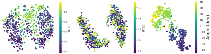
The image presents three scatter plots arranged horizontally. Each plot displays a relationship between two variables, RT60 and an Angle (in degrees), with a third variable represented by the color of each data point. The plots appear to visualize data from a single experiment or dataset, potentially showing how the angle and RT60 relate to each other under varying conditions.
### Components/Axes
Each plot shares the following components:
* **X-axis:** Labeled "RT60", with a scale ranging from approximately 0.2 to 1.0, with increments of 0.2.
* **Y-axis:** Labeled "Angle (deg)", with a scale ranging from approximately -40 to -10 degrees, with increments of 10.
* **Color Scale (Legend):** Positioned to the right of each plot. The scale represents a third variable, with colors ranging from purple (approximately 0.2) to yellow (approximately 1.0). The scale is labeled "RT60" despite being used to color the points.
* **Data Points:** Each plot contains a cloud of colored dots, representing individual data points.
### Detailed Analysis or Content Details
**Plot 1 (Leftmost):**
* The data points are distributed in a roughly circular pattern.
* The color gradient appears relatively uniform across the circle, with a slight concentration of purple points at the bottom and yellow points at the top.
* Approximate data points (estimated from visual inspection):
* RT60 ≈ 0.3, Angle ≈ -30 (Purple)
* RT60 ≈ 0.7, Angle ≈ -10 (Yellow)
* RT60 ≈ 0.5, Angle ≈ -20 (Green)
**Plot 2 (Center):**
* The data points are elongated vertically, forming a roughly teardrop shape.
* The color gradient shows a clear trend: points with lower RT60 values (purple) are concentrated at the bottom, while points with higher RT60 values (yellow) are concentrated at the top.
* Approximate data points:
* RT60 ≈ 0.3, Angle ≈ -35 (Purple)
* RT60 ≈ 0.8, Angle ≈ -10 (Yellow)
* RT60 ≈ 0.6, Angle ≈ -25 (Green)
**Plot 3 (Rightmost):**
* The data points are more clustered than in the previous plots, forming a roughly elliptical shape.
* The color gradient is similar to Plot 2, with lower RT60 values (purple) at the bottom and higher RT60 values (yellow) at the top.
* Approximate data points:
* RT60 ≈ 0.3, Angle ≈ -40 (Purple)
* RT60 ≈ 0.9, Angle ≈ -10 (Yellow)
* RT60 ≈ 0.7, Angle ≈ -20 (Green)
### Key Observations
* All three plots show a positive correlation between RT60 and Angle. As RT60 increases, the Angle tends to increase (become less negative).
* The distribution of data points varies significantly between the plots, suggesting different underlying conditions or groupings within the dataset.
* The color gradient consistently reflects the RT60 value, providing an additional dimension of information.
### Interpretation
The data suggests a relationship between RT60, Angle, and the color-coded variable (which is also RT60). RT60, often used in acoustics, represents the reverberation time of a space. The Angle, likely representing an incident or reflection angle, could be related to the direction of sound or a surface. The positive correlation indicates that as the reverberation time increases, the angle also increases.
The differences in the distribution of data points across the three plots could be due to:
* **Different experimental conditions:** Each plot might represent data collected under different settings (e.g., different room sizes, materials, or sound sources).
* **Subgroups within the data:** The data might be divided into distinct groups based on other factors not shown in the plots.
* **Noise or outliers:** Some plots might contain more noise or outliers than others, affecting the overall distribution.
The consistent color gradient reinforces the relationship between RT60 and the color variable, suggesting that the color is a reliable indicator of RT60 value. The plots provide a visual representation of how these variables interact, potentially aiding in the understanding of acoustic behavior in different environments.