# Technical Data Extraction: Conductance (G) vs. Spin-Orbit Coupling ($\lambda_I/t$)
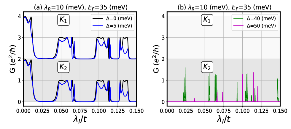
This document provides a comprehensive extraction of data and trends from the provided scientific plots. The image consists of two side-by-side panels, (a) and (b), showing the conductance $G$ as a function of the dimensionless parameter $\lambda_I/t$ for different values of $\Delta$.
## 1. Global Metadata and Axis Definitions
* **Common Parameters (Both Panels):**
* $\lambda_R = 10 \text{ (meV)}$
* $E_F = 35 \text{ (meV)}$
* **Y-Axis:** Conductance $G$ in units of $(e^2/h)$.
* **Range:** 0 to 4.
* **Major Tick Marks:** 0, 1, 2, 3, 4.
* **X-Axis:** Dimensionless parameter $\lambda_I/t$.
* **Range:** 0.000 to 0.150.
* **Major Tick Marks:** 0.000, 0.025, 0.050, 0.075, 0.100, 0.125, 0.150.
* **Internal Labels:** Both panels contain two distinct regions labeled $K_1$ (upper half, $G > 2$) and $K_2$ (lower half, $G < 2$).
---
## 2. Panel (a) Analysis
**Header:** (a) $\lambda_R=10 \text{ (meV)}, E_F=35 \text{ (meV)}$
### Legend and Series Identification
* **Location:** Top right quadrant of panel (a).
* **Series 1 (Black Line):** $\Delta = 0 \text{ (meV)}$
* **Series 2 (Blue Line):** $\Delta = 5 \text{ (meV)}$
### Trend Description and Data Points
Panel (a) shows high conductance plateaus interspersed with deep gaps where conductance drops to zero.
* **Region $K_1$ (Top):**
* **Trend:** Starts at $G=4$ at $\lambda_I/t = 0$. Both lines show a plateau until $\sim 0.010$, followed by a sharp drop to $G=2$ (the floor of the $K_1$ region).
* **Plateau 1 ($\sim 0.050$ to $0.065$):** Black line reaches $G=3$. Blue line is slightly lower with oscillations.
* **Plateau 2 ($\sim 0.100$ to $0.115$):** Black line reaches $G=3$. Blue line shows a significant dip in the middle of this range.
* **Plateau 3 ($\sim 0.130$ to $0.140$):** Black line reaches $G=3$. Blue line reaches $\sim 2.5$.
* **Region $K_2$ (Bottom):**
* **Trend:** Mirrors the $K_1$ behavior but shifted down by 2 units. Starts at $G=2$.
* **Gaps:** Conductance drops to $G=0$ between $0.015-0.045$, $0.070-0.095$, and $0.115-0.125$.
* **Effect of $\Delta$:** Increasing $\Delta$ from 0 to 5 meV (Blue line) generally suppresses the conductance peaks and introduces more oscillatory behavior within the plateaus.
---
## 3. Panel (b) Analysis
**Header:** (b) $\lambda_R=10 \text{ (meV)}, E_F=35 \text{ (meV)}$
### Legend and Series Identification
* **Location:** Top right quadrant of panel (b).
* **Series 3 (Green Line):** $\Delta = 40 \text{ (meV)}$
* **Series 4 (Magenta Line):** $\Delta = 50 \text{ (meV)}$
### Trend Description and Data Points
Panel (b) shows a "suppressed" state. The $K_1$ region (top half) is entirely empty ($G=0$). All activity is confined to the $K_2$ region (bottom half) and consists of sharp, narrow spikes rather than broad plateaus.
* **Region $K_1$ (Top):**
* **Trend:** Constant $G=0$ for both series across the entire x-axis range.
* **Region $K_2$ (Bottom):**
* **Series 3 (Green):** Shows clusters of sharp spikes.
* Cluster 1: $\sim 0.020 - 0.025$, peak $G \approx 1.6$.
* Cluster 2: $\sim 0.055 - 0.065$, peak $G \approx 1.4$.
* Cluster 3: $\sim 0.105 - 0.110$, peak $G \approx 1.3$.
* Cluster 4: $\sim 0.145 - 0.150$, peak $G \approx 1.3$.
* **Series 4 (Magenta):** Shows even fewer and narrower spikes.
* Spike 1: $\sim 0.035$, very low $G$.
* Spike 2: $\sim 0.065$, $G \approx 0.5$.
* Spike 3: $\sim 0.075$, $G \approx 0.5$.
* Spike 4: $\sim 0.100$, $G \approx 1.3$.
* Spike 5: $\sim 0.115$, $G \approx 1.4$.
* Spike 6: $\sim 0.120$, $G \approx 0.7$.
---
## 4. Summary of Observations
1. **Phase Transition:** There is a clear transition between panel (a) and (b). Low $\Delta$ (0-5 meV) allows for broad conductance plateaus and transport in both $K_1$ and $K_2$ regimes. High $\Delta$ (40-50 meV) destroys the $K_1$ transport and reduces $K_2$ transport to isolated resonance spikes.
2. **Symmetry:** The $K_1$ and $K_2$ regions in panel (a) are mathematically related by a vertical shift of 2 units ($G_{K1} = G_{K2} + 2$).
3. **Impact of $\Delta$:** Increasing the $\Delta$ parameter acts as a gap-opening mechanism that suppresses the total conductance and eventually localizes the transport into narrow energy/coupling windows.