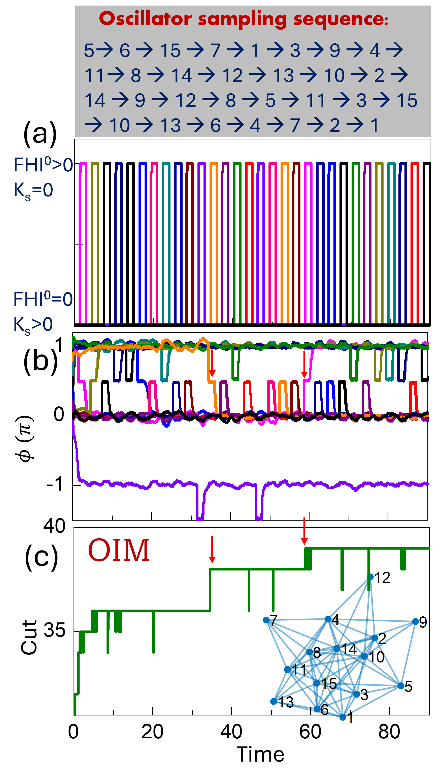
## [Diagram]: Oscillator Sampling and Optimization Dynamics ### Overview This image presents a multi-panel technical figure (labeled a, b, and c) illustrating the dynamics of an oscillator-based system, likely used for solving combinatorial optimization problems (such as the Max-Cut problem). The figure includes a specific sampling sequence, a binary state switching plot, a phase evolution plot, and a "Cut" value optimization plot featuring an inset network graph. ### Components/Axes * **Top Text Block:** "Oscillator sampling sequence:" followed by a sequence of numbers. * **Panel (a):** A pulse train/square wave plot. * **Y-axis:** Binary states. Top label: "FHI⁰>0, K_s=0"; Bottom label: "FHI⁰=0, K_s>0". * **Panel (b):** A time-series plot. * **Y-axis:** $\phi$ ($\pi$). Scale ranges from -1 to 1. * **X-axis:** Shared "Time" axis (0 to 80+). * **Panel (c):** A step-function plot. * **Y-axis:** "Cut". Scale ranges from 35 to 40. * **X-axis:** "Time". * **Inset:** A network graph with nodes labeled 1 through 15. * **Annotations:** Red arrows appear in panels (b) and (c) at approximately Time = 35 and Time = 60. ### Detailed Analysis #### 1. Oscillator Sampling Sequence The sequence is provided as follows: 5 $\rightarrow$ 6 $\rightarrow$ 15 $\rightarrow$ 7 $\rightarrow$ 1 $\rightarrow$ 3 $\rightarrow$ 9 $\rightarrow$ 4 $\rightarrow$ 11 $\rightarrow$ 8 $\rightarrow$ 14 $\rightarrow$ 12 $\rightarrow$ 13 $\rightarrow$ 10 $\rightarrow$ 2 $\rightarrow$ 14 $\rightarrow$ 9 $\rightarrow$ 12 $\rightarrow$ 8 $\rightarrow$ 5 $\rightarrow$ 11 $\rightarrow$ 3 $\rightarrow$ 15 $\rightarrow$ 10 $\rightarrow$ 13 $\rightarrow$ 6 $\rightarrow$ 4 $\rightarrow$ 7 $\rightarrow$ 2 $\rightarrow$ 1 #### 2. Panel (a): Switching States This panel displays a high-frequency square wave. The signal alternates between two states: * **State 1 (Top):** FHI⁰ > 0, K_s = 0 * **State 2 (Bottom):** FHI⁰ = 0, K_s > 0 The transitions are perfectly synchronized, indicating a switching mechanism between two distinct operational modes or parameters. #### 3. Panel (b): Phase Evolution ($\phi$) This plot tracks the phase ($\phi$) of multiple oscillators over time. * **Trend:** Most lines oscillate or remain near 0. * **Outlier:** One distinct purple line drops sharply from 0 to -1 at the very beginning (Time $\approx$ 0) and remains at -1 for the duration of the plot. * **Dynamics:** There are periodic spikes and transitions in the other colored lines. Two specific time points (marked by red arrows at Time $\approx$ 35 and Time $\approx$ 60) show distinct phase shifts or re-alignments. #### 4. Panel (c): Cut Optimization and Network Graph * **Main Plot:** A green line representing the "Cut" value. The value starts at approximately 34, increases in steps, and reaches 40. * **Step Increases:** The "Cut" value increases at specific intervals. Notably, the red arrows at Time $\approx$ 35 and Time $\approx$ 60 align with the upward steps in the "Cut" value. * **Inset Network Graph:** Located in the bottom-right. It depicts a graph with 15 nodes (labeled 1-15). The nodes are interconnected by a dense web of blue lines (edges). The graph appears to be a complete or near-complete graph, representing the structure being optimized. ### Key Observations * **Correlation:** The red arrows in panels (b) and (c) are vertically aligned. This suggests that the phase shifts observed in panel (b) are the direct cause of the increases in the "Cut" value in panel (c). * **Optimization Progress:** The "Cut" value increases over time, suggesting an iterative optimization process (OIM - likely "Oscillator-based Ising Machine" or "Oscillator-based Optimization Method") that improves the solution quality as the system evolves. * **System Stability:** The purple line in panel (b) suggests that one oscillator (or a subset) locks into a stable phase of -1, while others remain dynamic. ### Interpretation This figure demonstrates the operational mechanics of an oscillator-based computing system solving a graph optimization problem (specifically, the Max-Cut problem). 1. **The Process:** The system uses a specific sampling sequence to update oscillators. 2. **The Mechanism:** Panel (a) shows the system switching between two modes (FHI and K_s), which likely controls the coupling strength or the Hamiltonian parameters of the system. 3. **The Result:** As the system evolves, the oscillators adjust their phases (panel b). When the system reaches specific states (indicated by the red arrows), the "Cut" value—a metric of the optimization quality—increases (panel c). 4. **The Goal:** The system is attempting to maximize the "Cut" value, which corresponds to finding the optimal partition of the network graph shown in the inset. The step-wise increase indicates that the system is successfully finding better solutions over time.