TECHNICAL ASSET FINGERPRINT
94a1fc47f1f29e4656caa077
Click to view fullscreen
Press ESC or click to close
FOUND IN PAPERS
EXPERT: gemini-2.5-flash-free VERSION 1
RUNTIME: google-free/gemini-2.5-flash
INTEL_VERIFIED
## Chart Type: Heatmap of Performance Metric vs. Program Parameters
### Overview
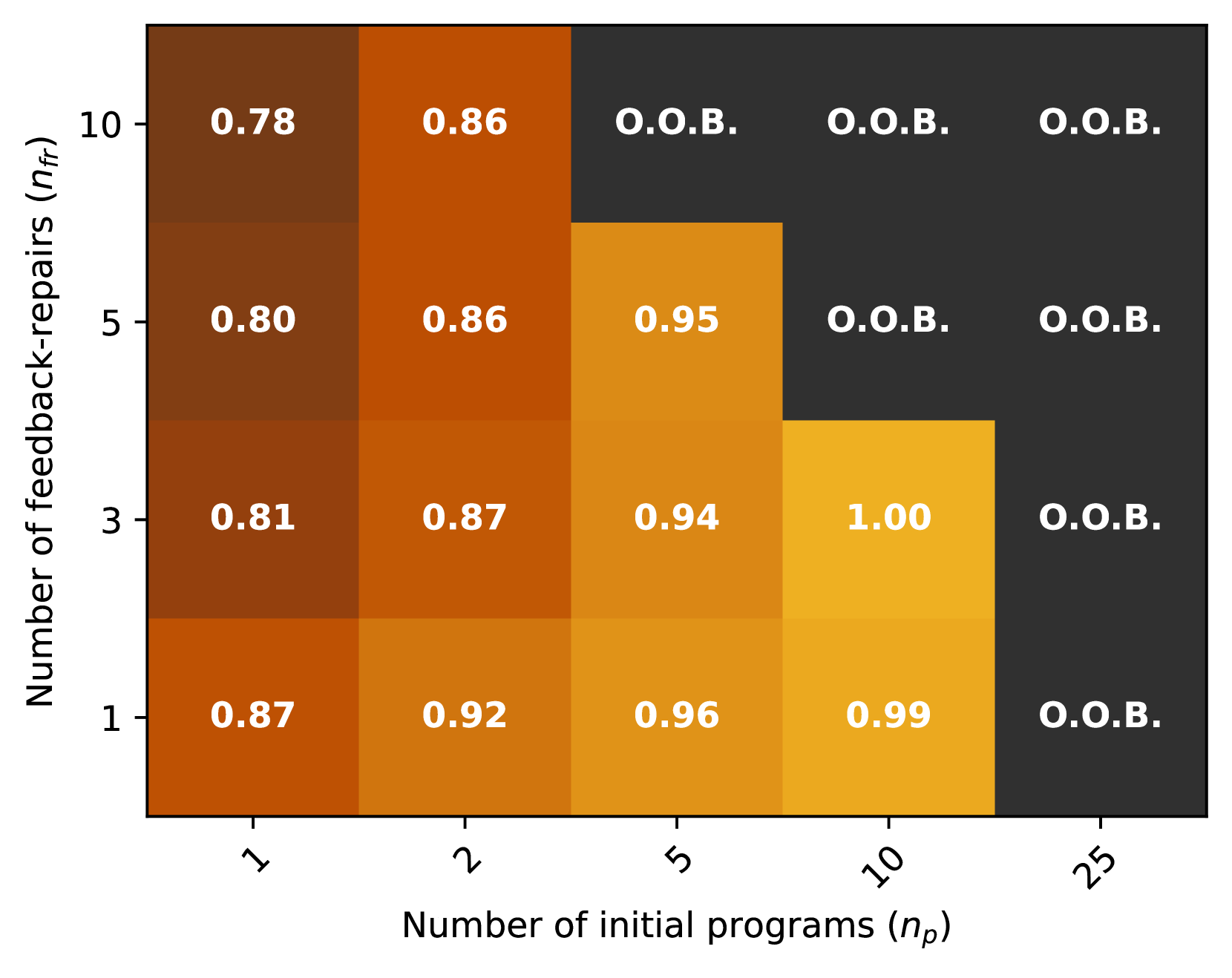
This image displays a heatmap illustrating a performance metric (likely a success rate or accuracy, ranging from 0.78 to 1.00) across different combinations of two parameters: "Number of initial programs ($n_p$)" and "Number of feedback-repairs ($n_{fr}$)". The cells are color-coded, with darker brown indicating lower values and brighter yellow indicating higher values. A significant portion of the grid, particularly in the upper-right, is marked "O.O.B." (Out Of Bounds) and colored dark grey, indicating conditions where a numerical result was not obtained.
### Components/Axes
The chart is a 2D grid with two categorical axes:
* **Y-axis (left side)**: Labeled "Number of feedback-repairs ($n_{fr}$)".
* Tick markers (from bottom to top): 1, 3, 5, 10.
* **X-axis (bottom side)**: Labeled "Number of initial programs ($n_p$)".
* Tick markers (from left to right): 1, 2, 5, 10, 25.
There is no explicit color legend. However, the color intensity within the cells implicitly represents the numerical values:
* Darkest brown: Corresponds to values around 0.78.
* Medium brown/orange: Corresponds to values around 0.80 to 0.92.
* Lighter orange/yellow: Corresponds to values around 0.94 to 0.99.
* Brightest yellow: Corresponds to the value 1.00.
* Dark grey: Corresponds to "O.O.B." entries.
### Detailed Analysis
The heatmap is a 4x5 grid, with rows corresponding to $n_{fr}$ values and columns corresponding to $n_p$ values. Each cell contains a numerical value (formatted to two decimal places) or the text "O.O.B.".
**Data Table (Values in cells, with qualitative color description):**
| $n_{fr}$ \ $n_p$ | 1 (Dark Brown) | 2 (Medium Brown/Orange) | 5 (Lighter Orange/Yellow) | 10 (Lighter Orange/Yellow) | 25 (Dark Grey) |
| :--------------- | :------------- | :---------------------- | :------------------------ | :------------------------- | :------------- |
| **10** | 0.78 | 0.86 | O.O.B. | O.O.B. | O.O.B. |
| **5** | 0.80 | 0.86 | 0.95 | O.O.B. | O.O.B. |
| **3** | 0.81 | 0.87 | 0.94 | 1.00 | O.O.B. |
| **1** | 0.87 | 0.92 | 0.96 | 0.99 | O.O.B. |
**Trends and Observations by Row (increasing $n_p$ for fixed $n_{fr}$):**
* **For $n_{fr}=10$**: Values increase from 0.78 (dark brown) to 0.86 (medium brown/orange), then transition to "O.O.B." (dark grey) for $n_p=5, 10, 25$.
* **For $n_{fr}=5$**: Values increase from 0.80 (dark brown) to 0.86 (medium brown/orange) to 0.95 (lighter orange/yellow), then transition to "O.O.B." (dark grey) for $n_p=10, 25$.
* **For $n_{fr}=3$**: Values increase from 0.81 (dark brown) to 0.87 (medium brown/orange) to 0.94 (lighter orange/yellow) to 1.00 (brightest yellow), then transition to "O.O.B." (dark grey) for $n_p=25$.
* **For $n_{fr}=1$**: Values consistently increase from 0.87 (medium brown/orange) to 0.92 (medium brown/orange) to 0.96 (lighter orange/yellow) to 0.99 (lighter orange/yellow), then transition to "O.O.B." (dark grey) for $n_p=25$.
**Trends and Observations by Column (increasing $n_{fr}$ for fixed $n_p$):**
* **For $n_p=1$**: Values generally decrease from 0.87 (medium brown/orange) to 0.81 (dark brown) to 0.80 (dark brown) to 0.78 (dark brown).
* **For $n_p=2$**: Values show a slight decrease then stability: 0.92 (medium brown/orange) to 0.87 (medium brown/orange) to 0.86 (medium brown/orange) to 0.86 (medium brown/orange).
* **For $n_p=5$**: Values show a slight decrease then increase: 0.96 (lighter orange/yellow) to 0.94 (lighter orange/yellow) to 0.95 (lighter orange/yellow), then transition to "O.O.B." (dark grey) for $n_{fr}=10$.
* **For $n_p=10$**: Values increase from 0.99 (lighter orange/yellow) to 1.00 (brightest yellow), then transition to "O.O.B." (dark grey) for $n_{fr}=5, 10$.
* **For $n_p=25$**: All values are "O.O.B." (dark grey).
### Key Observations
* The highest performance value observed is 1.00, located at $n_p=10$ and $n_{fr}=3$. This cell is colored the brightest yellow.
* The lowest performance value observed is 0.78, located at $n_p=1$ and $n_{fr}=10$. This cell is colored the darkest brown.
* Generally, increasing the "Number of initial programs ($n_p$)" tends to improve the performance metric for a given "Number of feedback-repairs ($n_{fr}$)", up to a certain point.
* Increasing the "Number of feedback-repairs ($n_{fr}$)" tends to decrease performance when the "Number of initial programs ($n_p$)" is low (e.g., $n_p=1, 2$).
* The "O.O.B." region occupies the top-right portion of the heatmap, forming a triangular pattern. This indicates that combinations with a high number of initial programs and/or a high number of feedback-repairs lead to "Out Of Bounds" conditions. Specifically, $n_p=25$ always results in "O.O.B.", and for $n_p=10$, $n_{fr}$ values of 5 and 10 result in "O.O.B.". For $n_p=5$, $n_{fr}=10$ results in "O.O.B.".
### Interpretation
The heatmap likely represents the results of an experiment or simulation where the performance of a system or algorithm is evaluated based on two configurable parameters: the number of initial programs and the number of feedback-repairs. The numerical values (0.78 to 1.00) are a measure of success or efficiency, with higher values being better.
The term "O.O.B." (Out Of Bounds) suggests that for these parameter combinations, the system either failed to produce a result, exceeded a computational budget (time, memory), or fell outside a predefined operational range. This implies a constraint or limitation in the system's ability to handle certain configurations.
The data suggests a sweet spot for performance. While increasing the "Number of initial programs ($n_p$)" generally improves the metric, it also increases the likelihood of hitting an "O.O.B." condition, especially when combined with a higher "Number of feedback-repairs ($n_{fr}$)". Conversely, a very low "Number of initial programs ($n_p=1$)" consistently yields lower performance, regardless of feedback-repairs.
The optimal observed performance (1.00) is achieved with a moderate number of initial programs ($n_p=10$) and a relatively low number of feedback-repairs ($n_{fr}=3$). This indicates that beyond a certain point, additional feedback-repairs might not be beneficial or could even be detrimental, particularly when combined with a large number of initial programs, leading to the "O.O.B." state. The "O.O.B." region highlights the practical limits or computational costs associated with scaling these parameters. Researchers or engineers using this data would likely aim for parameter combinations within the high-performance, non-"O.O.B." region, balancing performance with resource constraints.
DECODING INTELLIGENCE...