## 3D Surface Plot: Minimised Energy vs. θ1 and θ2 ### Overview The image is a 3D surface plot visualizing the relationship between "Minimised Energy" and two variables, θ1 and θ2. The surface is colored to represent the energy levels, with lower energy values appearing in purple/blue and higher energy values in yellow/green. The plot shows a complex energy landscape with a minimum point and varying degrees of curvature. ### Components/Axes * **X-axis:** θ1, ranging from approximately -5 to 5. Axis markers are present at -4, -2, 0, 2, and 4. * **Y-axis:** θ2, ranging from approximately -5 to 5. Axis markers are present at -4, -2, 0, 2, and 4. * **Z-axis:** Minimised Energy, ranging from -0.14 to -0.02. Axis markers are present at -0.14, -0.12, -0.10, -0.08, -0.06, -0.04, and -0.02. ### Detailed Analysis The surface plot shows the following trends: * **General Shape:** The surface has a valley-like structure, indicating a region of lower energy. There is a clear minimum point in this valley. * **Energy Minimum:** The minimum energy value appears to be around -0.14, located near θ1 = 0 and θ2 = 0. * **Energy Peaks:** There are two peaks in the energy surface, one on each side of the valley along the θ2 axis. The peaks reach a maximum energy of approximately -0.02. * **Symmetry:** The plot appears to be roughly symmetrical with respect to the θ1 axis. ### Key Observations * The plot clearly shows a minimum energy configuration for the system being modeled. * The energy landscape is not uniform, with significant variations depending on the values of θ1 and θ2. * The presence of peaks suggests that there are other, less stable, configurations. ### Interpretation The 3D surface plot visualizes an energy landscape, likely representing a system where the energy is dependent on two parameters, θ1 and θ2. The plot demonstrates that there is a specific combination of θ1 and θ2 that minimizes the energy of the system. The shape of the surface indicates the sensitivity of the energy to changes in these parameters. The presence of peaks suggests that there may be other local minima or saddle points in the energy landscape, which could correspond to metastable states of the system. The plot is useful for understanding the stability and behavior of the system as a function of θ1 and θ2.

\n ## 3D Surface Plot: Minimized Energy Landscape ### Overview The image presents a 3D surface plot visualizing a minimized energy landscape. The plot depicts the relationship between two parameters, θ₁ and θ₂, and their corresponding minimized energy value. The surface is colored to represent varying energy levels, with cooler colors (greens and blues) indicating lower energy and warmer colors (yellows and reds) indicating higher energy. ### Components/Axes * **X-axis:** θ₁ ranging from approximately -4 to 4. * **Y-axis:** θ₂ ranging from approximately -4 to 4. * **Z-axis:** Minimized Energy ranging from approximately -0.14 to -0.02. * **Surface:** Represents the minimized energy as a function of θ₁ and θ₂. * **Color Gradient:** A continuous color gradient is used to represent the energy levels. The gradient appears to transition from purple (lowest energy) to green, yellow, and finally to a lighter shade of green/yellow (highest energy). ### Detailed Analysis The surface exhibits two distinct minima (valleys). * **Left Minimum:** Located around θ₁ ≈ -4 and θ₂ ≈ 2, with a minimized energy of approximately -0.13 to -0.14. The surface rises relatively steeply on either side of this minimum. * **Right Minimum:** Located around θ₁ ≈ 4 and θ₂ ≈ -2, with a minimized energy of approximately -0.13 to -0.14. Similar to the left minimum, the surface rises steeply around this point. * **Central Ridge:** A ridge of higher energy (yellow/green) runs between the two minima, peaking around θ₁ ≈ 0 and θ₂ ≈ 0, with a minimized energy of approximately -0.02 to -0.04. * **Symmetry:** The plot appears roughly symmetric about the line θ₁ = θ₂ = 0, although there are subtle differences in the shape of the surface around each minimum. ### Key Observations * The energy landscape has multiple local minima, suggesting the possibility of multiple stable states. * The steepness of the surface around the minima indicates that small changes in θ₁ or θ₂ can lead to significant changes in energy. * The central ridge represents an unstable state, as any small perturbation would likely cause the system to move towards one of the minima. ### Interpretation This plot likely represents the result of an optimization process or a simulation of a physical system. The two minima suggest two possible stable configurations or states of the system. The energy values at these minima indicate the relative stability of each state. The shape of the surface and the presence of the central ridge provide information about the energy barriers between the different states. The plot demonstrates a complex energy landscape with multiple potential energy wells. This type of landscape is common in many physical and chemical systems, and understanding its features is crucial for predicting the behavior of the system. The visualization allows for a quick assessment of the system's stability and the ease with which it can transition between different states. The data suggests that the system will tend to settle into one of the two minima, but the specific state it reaches may depend on initial conditions and external factors.

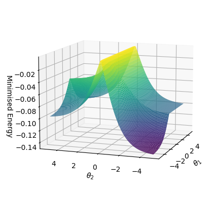
## 3D Surface Plot: Minimised Energy Landscape ### Overview The image displays a three-dimensional surface plot visualizing a function of two variables, θ₁ and θ₂. The plot represents an "energy landscape," where the vertical axis shows the "Minimised Energy" value. The surface is colored according to its height (energy value), creating a topographical map of the function's behavior across the parameter space. ### Components/Axes * **Chart Type:** 3D Surface Plot. * **Vertical Axis (Z-axis):** * **Label:** "Minimised Energy" * **Scale:** Linear, ranging from approximately -0.14 at the bottom to -0.02 at the top. * **Markers:** Ticks are present at intervals of 0.02 (e.g., -0.14, -0.12, -0.10, -0.08, -0.06, -0.04, -0.02). * **Horizontal Axes (X and Y axes):** * **Axis 1 (Right side, receding into the distance):** Labeled "θ₁". Scale ranges from -4 to 4, with major ticks at -4, -2, 0, 2, 4. * **Axis 2 (Left side, foreground):** Labeled "θ₂". Scale ranges from -4 to 4, with major ticks at -4, -2, 0, 2, 4. * **Color Mapping:** The surface uses a continuous color gradient (a "heatmap" applied to the 3D surface) to represent the Z-axis (Energy) value. * **Yellow/Light Green:** Corresponds to higher (less negative) energy values, near the top of the scale (~ -0.02 to -0.04). * **Green/Teal:** Corresponds to mid-range energy values (~ -0.06 to -0.08). * **Blue/Purple:** Corresponds to lower (more negative) energy values, near the bottom of the scale (~ -0.10 to -0.14). * **Grid:** A wireframe grid is plotted on the surface, following the contours of the function and aligning with the θ₁ and θ₂ axes, aiding in depth perception and value estimation. * **Perspective:** The plot is viewed from an angled perspective, looking down onto the surface from a position where both θ₁ and θ₂ axes are visible. ### Detailed Analysis * **Surface Topology:** The surface is not flat; it exhibits significant curvature with distinct peaks, valleys, and saddle points. * **General Trend:** The energy value generally decreases (becomes more negative) as one moves away from the central region (θ₁ ≈ 0, θ₂ ≈ 0) towards the edges of the plotted domain, particularly along the θ₂ axis. * **Key Features:** 1. **Central Ridge/Saddle Point:** There is a prominent ridge or saddle point structure near the center of the plot (θ₁ ≈ 0, θ₂ ≈ 0). The energy here is relatively high (yellow/green, approx. -0.04 to -0.06). 2. **Deep Valley along θ₂:** A pronounced, deep valley runs roughly parallel to the θ₂ axis. The lowest energy points (dark purple, approx. -0.12 to -0.14) are found in this valley, which appears to be centered around θ₂ ≈ -2 to -4, extending across a range of θ₁ values. 3. **Secondary Valley/Depression:** Another region of lower energy (blue/purple) is visible on the far side of the central ridge, suggesting a second, possibly shallower, valley. 4. **Asymmetry:** The landscape is not symmetric. The descent into the primary valley along negative θ₂ is steeper and deeper than the changes observed along the θ₁ axis. ### Key Observations * The function being plotted has multiple local minima (the valleys) and at least one saddle point (the central ridge). * The global minimum within this visible window appears to be located in the deep valley at negative θ₂ values. * The color gradient effectively highlights the steepness of the slopes; rapid color changes indicate steep gradients in the energy function. * The grid lines become densely packed in the steep valley regions, visually confirming the high rate of change. ### Interpretation This plot visualizes the solution space of an optimization or physical system where "Minimised Energy" is the objective function to be minimized with respect to two parameters, θ₁ and θ₂. * **What it demonstrates:** The landscape shows that finding the lowest energy state is non-trivial. A simple gradient descent algorithm starting from the central region (θ₁≈0, θ₂≈0) could get trapped on the saddle point or roll into one of the valleys depending on the initial direction. The deep valley at negative θ₂ represents the most stable (lowest energy) configuration for the system within the explored parameter range. * **Relationship between elements:** The θ₁ and θ₂ parameters are coupled; the energy value depends on a specific combination of both, not on each independently. The shape of the valleys and ridges defines this coupling. * **Notable Anomalies/Patterns:** The most striking pattern is the dominant, deep valley aligned with the θ₂ axis. This suggests that the system's energy is more sensitive to changes in θ₂ than to changes in θ₁, especially in the negative θ₂ region. The saddle point indicates an unstable equilibrium—a small perturbation would cause the system to "roll down" into one of the adjacent valleys. This type of landscape is common in problems involving molecular conformations, machine learning loss functions, or control system stability analysis.

## 3D Surface Plot: Minimised Energy Landscape ### Overview The image depicts a 3D surface plot visualizing a minimised energy landscape as a function of two angular variables, θ₁ and θ₂. The plot uses a color gradient (purple to yellow) to represent energy values, with a grid overlay for spatial reference. The surface exhibits multiple peaks, troughs, and saddle points, suggesting a complex energy distribution. ### Components/Axes - **X-axis (θ₂)**: Ranges from -4 to 4, labeled with increments of 2. - **Y-axis (θ₁)**: Ranges from -4 to 4, labeled with increments of 2. - **Z-axis (Minimised Energy)**: Ranges from -0.14 to -0.02, with increments of 0.02. - **Color Gradient**: - Purple (low energy, ~-0.14) to Yellow (high energy, ~-0.02). - No explicit legend, but color intensity correlates with energy values. - **Grid**: 3D grid lines in gray, providing spatial context for the surface. ### Detailed Analysis 1. **Peaks**: - **Highest Peak**: Located at θ₂ ≈ 0, θ₁ ≈ 0, with energy ≈ -0.02 (yellow region). - **Secondary Peak**: Near θ₂ ≈ 2, θ₁ ≈ 2, with energy ≈ -0.04 (green-yellow transition). 2. **Troughs**: - **Deepest Trough**: At θ₂ ≈ -4, θ₁ ≈ -4, with energy ≈ -0.14 (dark purple). - **Secondary Trough**: Near θ₂ ≈ -2, θ₁ ≈ 2, with energy ≈ -0.08 (blue-green). 3. **Saddle Point**: - A critical point at θ₂ ≈ 2, θ₁ ≈ 2, where the surface transitions from rising to falling in orthogonal directions. 4. **Surface Shape**: - The plot resembles a "double-well" potential with asymmetric wells, influenced by the interaction between θ₁ and θ₂. ### Key Observations - The energy landscape is non-uniform, with localized minima and maxima. - The saddle point at (2, 2) suggests a critical configuration where small perturbations could lead to transitions between states. - Energy values are consistently negative, indicating a bounded system (e.g., potential energy relative to a reference). ### Interpretation This plot likely represents a **potential energy surface** in a physical or optimization context. The double-well structure implies multiple stable states (minima) separated by an energy barrier (saddle point). The asymmetry in well depths suggests preferential stability in certain configurations (e.g., θ₂ ≈ -4, θ₁ ≈ -4). The color gradient confirms that energy values are directly proportional to surface height, with no anomalies in the mapping. The plot could model phenomena such as molecular conformations, mechanical stability, or parameter optimization landscapes.