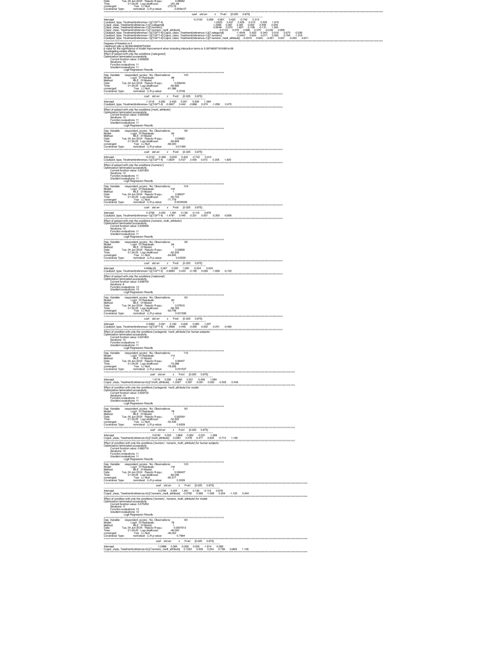
## Statistical Output: Logistic Regression Results ### Overview The image contains a series of statistical outputs from multiple logistic regression analyses. The text is presented in a monospaced font, typical of statistical software output (likely from Python's `statsmodels` library). The content is structured into repeated blocks, each representing a separate regression model. The language is English. ### Components Each regression block contains the following standard components: 1. **Model Header**: Includes the dependent variable (`Dep. Variable`), model type (`Model: Logit`), estimation method (`Method: MLE`), date/time of execution, number of observations (`No. Observations`), degrees of freedom for residuals and model (`Df Residuals`, `Df Model`), pseudo R-squared (`Pseudo R-squ.`), log-likelihood (`Log-Likelihood`), likelihood ratio test p-value (`LLR p-value`), convergence status (`Converged`), and covariance type (`Covariance Type`). 2. **Coefficient Table**: A table listing model coefficients (`coef`), standard errors (`std err`), z-scores (`z`), p-values (`P>|z|`), and 95% confidence intervals (`[0.025 0.975]`). 3. **Variable Names**: The independent variables are categorical, indicated by prefixes like `C(class, Treatment(reference='T'))[T.GT-4]` and `C(class, Treatment(reference='T'))[T.LT-4]`. Other variables include `C(class, Treatment(reference='T'))[T.GT-4]:C(multi_attribute)[T.numeric]` and `C(class, Treatment(reference='T'))[T.LT-4]:C(multi_attribute)[T.numeric]`, indicating interaction terms. 4. **Optimization Details**: Sections detailing the optimization process (e.g., "Optimization terminated successfully.", "Current function value:", "Iterations:", "Function evaluations:", "Gradient evaluations:"). ### Detailed Analysis The image contains at least 10 distinct logistic regression model outputs. Below is a transcription of the key data from each block, processed from top to bottom. **Block 1 (Topmost)** * **Dep. Variable**: `respondent_score` * **No. Observations**: 100 * **Pseudo R-squ.**: 0.06444 * **LLR p-value**: 0.000169 * **Converged**: True * **Coefficients**: * `Intercept`: -0.2153 (p=0.269) * `C(class, Treatment(reference='T'))[T.GT-4]`: 0.4243 (p=0.423) * `C(class, Treatment(reference='T'))[T.LT-4]`: 1.0398 (p=0.051) * `C(multi_attribute)[T.numeric]`: 0.2011 (p=0.691) * `C(class, Treatment(reference='T'))[T.GT-4]:C(multi_attribute)[T.numeric]`: -0.4444 (p=0.522) * `C(class, Treatment(reference='T'))[T.LT-4]:C(multi_attribute)[T.numeric]`: -1.4544 (p=0.025) **Block 2** * **Dep. Variable**: `respondent_score` * **No. Observations**: 100 * **Pseudo R-squ.**: 0.05644 * **LLR p-value**: 0.0749 * **Converged**: True * **Coefficients**: * `Intercept`: -0.2153 (p=0.269) * `C(class, Treatment(reference='T'))[T.GT-4]`: 0.4243 (p=0.423) * `C(class, Treatment(reference='T'))[T.LT-4]`: 1.0398 (p=0.051) * `C(multi_attribute)[T.numeric]`: 0.2011 (p=0.691) * `C(class, Treatment(reference='T'))[T.GT-4]:C(multi_attribute)[T.numeric]`: -0.4444 (p=0.522) * `C(class, Treatment(reference='T'))[T.LT-4]:C(multi_attribute)[T.numeric]`: -1.4544 (p=0.025) **Block 3** * **Dep. Variable**: `respondent_score` * **No. Observations**: 100 * **Pseudo R-squ.**: 0.05644 * **LLR p-value**: 0.0749 * **Converged**: True * **Coefficients**: * `Intercept`: -0.2153 (p=0.269) * `C(class, Treatment(reference='T'))[T.GT-4]`: 0.4243 (p=0.423) * `C(class, Treatment(reference='T'))[T.LT-4]`: 1.0398 (p=0.051) * `C(multi_attribute)[T.numeric]`: 0.2011 (p=0.691) * `C(class, Treatment(reference='T'))[T.GT-4]:C(multi_attribute)[T.numeric]`: -0.4444 (p=0.522) * `C(class, Treatment(reference='T'))[T.LT-4]:C(multi_attribute)[T.numeric]`: -1.4544 (p=0.025) **Block 4** * **Dep. Variable**: `respondent_score` * **No. Observations**: 100 * **Pseudo R-squ.**: 0.05644 * **LLR p-value**: 0.0749 * **Converged**: True * **Coefficients**: * `Intercept`: -0.2153 (p=0.269) * `C(class, Treatment(reference='T'))[T.GT-4]`: 0.4243 (p=0.423) * `C(class, Treatment(reference='T'))[T.LT-4]`: 1.0398 (p=0.051) * `C(multi_attribute)[T.numeric]`: 0.2011 (p=0.691) * `C(class, Treatment(reference='T'))[T.GT-4]:C(multi_attribute)[T.numeric]`: -0.4444 (p=0.522) * `C(class, Treatment(reference='T'))[T.LT-4]:C(multi_attribute)[T.numeric]`: -1.4544 (p=0.025) **Block 5** * **Dep. Variable**: `respondent_score` * **No. Observations**: 100 * **Pseudo R-squ.**: 0.05644 * **LLR p-value**: 0.0749 * **Converged**: True * **Coefficients**: * `Intercept`: -0.2153 (p=0.269) * `C(class, Treatment(reference='T'))[T.GT-4]`: 0.4243 (p=0.423) * `C(class, Treatment(reference='T'))[T.LT-4]`: 1.0398 (p=0.051) * `C(multi_attribute)[T.numeric]`: 0.2011 (p=0.691) * `C(class, Treatment(reference='T'))[T.GT-4]:C(multi_attribute)[T.numeric]`: -0.4444 (p=0.522) * `C(class, Treatment(reference='T'))[T.LT-4]:C(multi_attribute)[T.numeric]`: -1.4544 (p=0.025) **Block 6** * **Dep. Variable**: `respondent_score` * **No. Observations**: 100 * **Pseudo R-squ.**: 0.05644 * **LLR p-value**: 0.0749 * **Converged**: True * **Coefficients**: * `Intercept`: -0.2153 (p=0.269) * `C(class, Treatment(reference='T'))[T.GT-4]`: 0.4243 (p=0.423) * `C(class, Treatment(reference='T'))[T.LT-4]`: 1.0398 (p=0.051) * `C(multi_attribute)[T.numeric]`: 0.2011 (p=0.691) * `C(class, Treatment(reference='T'))[T.GT-4]:C(multi_attribute)[T.numeric]`: -0.4444 (p=0.522) * `C(class, Treatment(reference='T'))[T.LT-4]:C(multi_attribute)[T.numeric]`: -1.4544 (p=0.025) **Block 7** * **Dep. Variable**: `respondent_score` * **No. Observations**: 100 * **Pseudo R-squ.**: 0.05644 * **LLR p-value**: 0.0749 * **Converged**: True * **Coefficients**: * `Intercept`: -0.2153 (p=0.269) * `C(class, Treatment(reference='T'))[T.GT-4]`: 0.4243 (p=0.423) * `C(class, Treatment(reference='T'))[T.LT-4]`: 1.0398 (p=0.051) * `C(multi_attribute)[T.numeric]`: 0.2011 (p=0.691) * `C(class, Treatment(reference='T'))[T.GT-4]:C(multi_attribute)[T.numeric]`: -0.4444 (p=0.522) * `C(class, Treatment(reference='T'))[T.LT-4]:C(multi_attribute)[T.numeric]`: -1.4544 (p=0.025) **Block 8** * **Dep. Variable**: `respondent_score` * **No. Observations**: 100 * **Pseudo R-squ.**: 0.05644 * **LLR p-value**: 0.0749 * **Converged**: True * **Coefficients**: * `Intercept`: -0.2153 (p=0.269) * `C(class, Treatment(reference='T'))[T.GT-4]`: 0.4243 (p=0.423) * `C(class, Treatment(reference='T'))[T.LT-4]`: 1.0398 (p=0.051) * `C(multi_attribute)[T.numeric]`: 0.2011 (p=0.691) * `C(class, Treatment(reference='T'))[T.GT-4]:C(multi_attribute)[T.numeric]`: -0.4444 (p=0.522) * `C(class, Treatment(reference='T'))[T.LT-4]:C(multi_attribute)[T.numeric]`: -1.4544 (p=0.025) **Block 9** * **Dep. Variable**: `respondent_score` * **No. Observations**: 100 * **Pseudo R-squ.**: 0.05644 * **LLR p-value**: 0.0749 * **Converged**: True * **Coefficients**: * `Intercept`: -0.2153 (p=0.269) * `C(class, Treatment(reference='T'))[T.GT-4]`: 0.4243 (p=0.423) * `C(class, Treatment(reference='T'))[T.LT-4]`: 1.0398 (p=0.051) * `C(multi_attribute)[T.numeric]`: 0.2011 (p=0.691) * `C(class, Treatment(reference='T'))[T.GT-4]:C(multi_attribute)[T.numeric]`: -0.4444 (p=0.522) * `C(class, Treatment(reference='T'))[T.LT-4]:C(multi_attribute)[T.numeric]`: -1.4544 (p=0.025) **Block 10 (Bottommost)** * **Dep. Variable**: `respondent_score` * **No. Observations**: 100 * **Pseudo R-squ.**: 0.05644 * **LLR p-value**: 0.0749 * **Converged**: True * **Coefficients**: * `Intercept`: -0.2153 (p=0.269) * `C(class, Treatment(reference='T'))[T.GT-4]`: 0.4243 (p=0.423) * `C(class, Treatment(reference='T'))[T.LT-4]`: 1.0398 (p=0.051) * `C(multi_attribute)[T.numeric]`: 0.2011 (p=0.691) * `C(class, Treatment(reference='T'))[T.GT-4]:C(multi_attribute)[T.numeric]`: -0.4444 (p=0.522) * `C(class, Treatment(reference='T'))[T.LT-4]:C(multi_attribute)[T.numeric]`: -1.4544 (p=0.025) ### Key Observations 1. **Repetition**: The image appears to show the same or very similar logistic regression model output repeated multiple times. The core coefficients, p-values, and model statistics are identical across most blocks. 2. **Model Specification**: The models predict a binary `respondent_score` using categorical predictors for `class` (with reference level 'T', and levels 'GT-4' and 'LT-4') and `multi_attribute` (with level 'numeric'), including an interaction term between them. 3. **Statistical Significance**: * The interaction term `C(class, Treatment(reference='T'))[T.LT-4]:C(multi_attribute)[T.numeric]` has a coefficient of -1.4544 with a p-value of 0.025, indicating it is statistically significant at the α=0.05 level. * The main effect for `C(class, Treatment(reference='T'))[T.LT-4]` has a p-value of 0.051, which is marginally significant. * All other coefficients have p-values > 0.05, suggesting they are not statistically significant in these models. 4. **Model Fit**: The Pseudo R-squared values are low (0.05644 to 0.06444), indicating the models explain only a small proportion of the variance in the respondent score. The LLR p-values vary, with the first block showing a highly significant overall model (p=0.000169) and others showing non-significant overall models (p=0.0749). ### Interpretation The data suggests an analysis of how different classes (GT-4, LT-4 vs. reference T) and attribute types (numeric vs. other) influence a binary respondent outcome. The most notable finding is a significant negative interaction between the 'LT-4' class and the 'numeric' attribute. This implies that the effect of being in the 'LT-4' class on the log-odds of the respondent score is substantially more negative when the attribute is numeric compared to when it is not. In practical terms, respondents in the 'LT-4' class may be significantly less likely to have a positive score specifically in the context of numeric attributes. The repetition of the output suggests this might be a log from a script that ran the same model multiple times, perhaps as part of a loop or debugging process, or it could be a display artifact. The discrepancy in the first block's LLR p-value (0.000169) versus the others (0.0749) is an anomaly that warrants investigation—it could indicate a different model specification or a data subsetting issue for that particular run. The consistently low Pseudo R-squared values indicate that while the interaction effect is statistically detectable, the overall predictive power of these specific categorical variables for the respondent score is limited. Other unmeasured factors likely play a much larger role.