\n
## Charts: Performance Comparison of Optimization Algorithms
### Overview
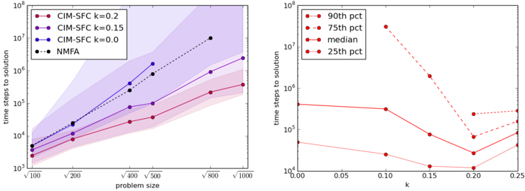
The image presents two charts comparing the performance of different optimization algorithms, specifically CIM-SFC with varying 'k' values and NMFA, in terms of time steps to solution. The left chart shows the relationship between time steps and problem size, while the right chart shows the relationship between time steps and the 'k' parameter.
### Components/Axes
**Left Chart:**
* **X-axis:** Problem Size (logarithmic scale, markers at 100, 200, √400 ≈ 20, √500 ≈ 22.4, 800, 1000)
* **Y-axis:** Time Steps to Solution (logarithmic scale, from 10^3 to 10^8)
* **Legend:**
* CIM-SFC k = 0.2 (Red circles with solid line)
* CIM-SFC k = 0.15 (Purple circles with solid line)
* CIM-SFC k = 0.0 (Blue circles with solid line)
* NMFA (Black dashed circles with dashed line)
**Right Chart:**
* **X-axis:** k (linear scale, from 0.00 to 0.25)
* **Y-axis:** Time Steps to Solution (logarithmic scale, from 10^3 to 10^7)
* **Legend:**
* 90th pct (Red circles with solid line)
* 75th pct (Red circles with dashed line)
* median (Blue circles with solid line)
* 25th pct (Red circles with dotted line)
### Detailed Analysis or Content Details
**Left Chart:**
* **CIM-SFC k = 0.2 (Red):** The line slopes upward, increasing from approximately 2.5 x 10^4 at problem size 100 to approximately 1.5 x 10^6 at problem size 1000.
* **CIM-SFC k = 0.15 (Purple):** The line slopes upward, increasing from approximately 1.5 x 10^4 at problem size 100 to approximately 8 x 10^5 at problem size 1000.
* **CIM-SFC k = 0.0 (Blue):** The line slopes upward, increasing from approximately 1 x 10^4 at problem size 100 to approximately 2 x 10^6 at problem size 1000.
* **NMFA (Black):** The line slopes upward, increasing from approximately 1.5 x 10^4 at problem size 100 to approximately 1.2 x 10^7 at problem size 1000.
**Right Chart:**
* **90th pct (Red, solid):** The line decreases sharply from approximately 6 x 10^6 at k = 0.00 to approximately 2 x 10^5 at k = 0.15, then increases slightly to approximately 3 x 10^5 at k = 0.25.
* **75th pct (Red, dashed):** The line decreases from approximately 2 x 10^6 at k = 0.00 to approximately 8 x 10^4 at k = 0.15, then remains relatively constant at approximately 6 x 10^4.
* **median (Blue, solid):** The line decreases from approximately 1.5 x 10^6 at k = 0.00 to approximately 2 x 10^4 at k = 0.15, then increases slightly to approximately 3 x 10^4 at k = 0.25.
* **25th pct (Red, dotted):** The line decreases sharply from approximately 5 x 10^5 at k = 0.00 to approximately 1 x 10^4 at k = 0.15, then increases to approximately 2 x 10^4 at k = 0.25.
### Key Observations
* In the left chart, NMFA consistently requires the most time steps to solution across all problem sizes.
* In the left chart, CIM-SFC with k=0.0 generally performs better than k=0.15 and k=0.2.
* In the right chart, all percentiles show a decrease in time steps as 'k' increases from 0.00 to 0.15, suggesting an optimal 'k' value around 0.15.
* In the right chart, the 90th percentile exhibits the highest time steps, indicating a wider range of performance variability.
### Interpretation
The data suggests that CIM-SFC is a more efficient optimization algorithm than NMFA, particularly for larger problem sizes. The 'k' parameter in CIM-SFC significantly impacts performance, with a value of 0.0 generally yielding the best results in terms of time steps to solution. However, the right chart indicates that there's an optimal range for 'k' (around 0.15) where performance is maximized. Beyond this point, increasing 'k' may lead to a slight increase in time steps, particularly for the 90th percentile, suggesting increased variability in performance. The difference between the 25th and 90th percentiles highlights the sensitivity of the algorithms to initial conditions or problem instances. The logarithmic scales on both axes emphasize the substantial differences in time steps required for different algorithms and parameter settings. The charts provide valuable insights for selecting the appropriate optimization algorithm and tuning its parameters for specific problem sizes and performance requirements.