## Chart Type: Comparative Line Graphs
### Overview
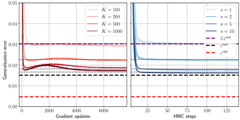
The image presents two line graphs side-by-side, comparing the generalization error of different models. The left graph shows the error as a function of gradient updates, with different lines representing different values of 'K'. The right graph shows the error as a function of HMC steps, with different lines representing different values of 's'. Both graphs also include horizontal dashed lines representing "2 ε<sup>uni</sup>" and "ε<sup>opt</sup>".
### Components/Axes
**Left Graph:**
* **X-axis:** "Gradient updates", ranging from 0 to 6000.
* **Y-axis:** "Generalisation error", ranging from 0.00 to 0.05.
* **Legend (top-right):**
* K = 100 (light red)
* K = 200 (red)
* K = 500 (dark red)
* K = 1000 (dark brown)
**Right Graph:**
* **X-axis:** "HMC steps", ranging from 0 to 125.
* **Y-axis:** "Generalisation error", ranging from 0.00 to 0.05.
* **Legend (top-right):**
* s = 1 (light blue)
* s = 2 (blue)
* s = 5 (dark blue)
* s = 10 (dark grey-blue)
**Shared Elements:**
* **Horizontal Dashed Lines:**
* 2 ε<sup>uni</sup> (purple, dashed) - Located at approximately y = 0.03 on both graphs.
* ε<sup>opt</sup> (red, dashed) - Located at approximately y = 0.005 on both graphs.
* ε<sup>opt</sup> (black, dashed) - Located at approximately y = 0.015 on both graphs.
### Detailed Analysis
**Left Graph (Gradient Updates):**
* **K = 100 (light red):** Starts at approximately 0.05, rapidly decreases to approximately 0.02, then slightly increases and stabilizes around 0.021 after 2000 gradient updates.
* **K = 200 (red):** Starts at approximately 0.05, rapidly decreases to approximately 0.02, then slightly increases and stabilizes around 0.020 after 2000 gradient updates.
* **K = 500 (dark red):** Starts at approximately 0.05, rapidly decreases to approximately 0.018, then slightly increases and stabilizes around 0.019 after 2000 gradient updates.
* **K = 1000 (dark brown):** Starts at approximately 0.05, rapidly decreases to approximately 0.017, then slightly increases and stabilizes around 0.018 after 2000 gradient updates.
**Right Graph (HMC Steps):**
* **s = 1 (light blue):** Starts at approximately 0.045, rapidly decreases to approximately 0.018, and stabilizes around 0.018 after 25 HMC steps.
* **s = 2 (blue):** Starts at approximately 0.04, rapidly decreases to approximately 0.016, and stabilizes around 0.016 after 25 HMC steps.
* **s = 5 (dark blue):** Starts at approximately 0.035, rapidly decreases to approximately 0.015, and stabilizes around 0.015 after 25 HMC steps.
* **s = 10 (dark grey-blue):** Starts at approximately 0.03, rapidly decreases to approximately 0.014, and stabilizes around 0.014 after 25 HMC steps.
### Key Observations
* In both graphs, the generalization error decreases rapidly in the initial steps (gradient updates or HMC steps) and then stabilizes.
* Higher values of 'K' (left graph) generally lead to lower generalization errors.
* Higher values of 's' (right graph) generally lead to lower generalization errors.
* The "2 ε<sup>uni</sup>" line represents an upper bound for the generalization error in both cases.
* The "ε<sup>opt</sup>" line represents a lower bound for the generalization error in both cases.
### Interpretation
The graphs illustrate the convergence behavior of different models during training. The left graph suggests that increasing 'K' (likely a parameter related to model complexity or data representation) improves the generalization performance, up to a point. The right graph suggests that increasing 's' (likely a parameter related to the sampling method) also improves generalization performance. The dashed lines provide benchmarks for the error, with "2 ε<sup>uni</sup>" representing a theoretical upper bound and "ε<sup>opt</sup>" representing an optimal error level. The fact that the error curves approach but do not consistently fall below "ε<sup>opt</sup>" suggests that there may be limitations to the models or training procedures used. The rapid initial decrease in error indicates efficient learning in the early stages of training.