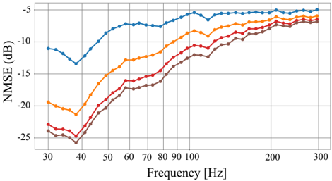
## Line Chart: NMSE vs. Frequency ### Overview The image presents a line chart illustrating the relationship between Frequency (in Hertz) and Normalized Mean Squared Error (NMSE) in decibels (dB). Four distinct data series are plotted, each represented by a different colored line. The chart appears to be evaluating the performance of a system or algorithm across a range of frequencies. ### Components/Axes * **X-axis:** Frequency [Hz], ranging from approximately 30 Hz to 300 Hz. Markers are present at 30, 40, 50, 60, 70, 80, 90, 100, 200, and 300 Hz. * **Y-axis:** NMSE (dB), ranging from approximately -25 dB to -5 dB. Markers are present at -5, -10, -15, -20, and -25 dB. * **Data Series:** Four lines, visually distinguishable by color: * Blue * Orange * Red * Dark Red/Brown ### Detailed Analysis Let's analyze each line individually, noting trends and approximate data points. * **Blue Line:** This line exhibits an upward sloping trend, starting at approximately -12 dB at 30 Hz and reaching approximately -4 dB at 300 Hz. It initially dips to around -14 dB at 40 Hz before steadily increasing. * **Orange Line:** This line also slopes upward, but starts at a lower NMSE value of approximately -20 dB at 30 Hz. It reaches approximately -6 dB at 300 Hz. It shows a more consistent upward trend than the blue line. * **Red Line:** This line begins at approximately -24 dB at 30 Hz and rises to approximately -10 dB at 300 Hz. It shows a relatively steep upward slope, particularly between 40 Hz and 100 Hz. * **Dark Red/Brown Line:** This line starts at approximately -25 dB at 30 Hz and increases to approximately -9 dB at 300 Hz. It has a similar upward trend to the red line, but consistently remains slightly below it. Here's a table summarizing approximate data points: | Frequency (Hz) | Blue Line (dB) | Orange Line (dB) | Red Line (dB) | Dark Red/Brown Line (dB) | |---|---|---|---|---| | 30 | -12 | -20 | -24 | -25 | | 40 | -14 | -16 | -18 | -19 | | 50 | -9 | -13 | -15 | -16 | | 60 | -7 | -11 | -13 | -14 | | 80 | -6 | -9 | -11 | -12 | | 100 | -5 | -8 | -10 | -10 | | 200 | -4 | -6 | -8 | -9 | | 300 | -4 | -6 | -10 | -9 | ### Key Observations * All four lines demonstrate a positive correlation between frequency and NMSE – as frequency increases, NMSE increases. * The dark red/brown line consistently exhibits the lowest performance (highest NMSE) at lower frequencies, but converges with the red line at higher frequencies. * The blue line consistently exhibits the best performance (lowest NMSE) across the entire frequency range. * The orange line falls between the blue and red lines in terms of performance. ### Interpretation The chart likely represents the performance of different noise reduction or signal processing algorithms across a range of frequencies. The NMSE metric indicates the error between the original signal and the processed signal. A lower NMSE value indicates better performance. The upward trend of all lines suggests that the algorithms become less effective at higher frequencies. The differences in performance between the lines indicate that some algorithms are more robust to frequency variations than others. The blue line's consistently lower NMSE suggests it is the most effective algorithm overall. The convergence of the red and dark red/brown lines at higher frequencies suggests that the performance difference between those algorithms diminishes as frequency increases. This could be due to limitations in the algorithms' ability to handle high-frequency components or due to the nature of the signal being processed. The data suggests that the choice of algorithm should be based on the frequency content of the signal. If the signal contains primarily low frequencies, the dark red/brown line algorithm might be sufficient. However, if the signal contains significant high-frequency components, the blue line algorithm would be the preferred choice.