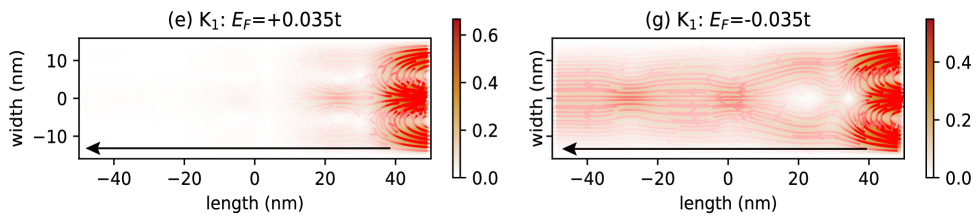
# Technical Data Extraction: Current Density Streamline Plots
This document provides a detailed technical extraction of the data and visual information contained in the provided image, which consists of two side-by-side heatmaps with overlaid streamlines, likely representing electron current flow in a nanostructure.
## 1. General Metadata
* **Language:** English
* **Image Type:** Scientific Heatmaps / Streamline Plots
* **Coordinate System:** Cartesian 2D (Length vs. Width)
* **Units:** Nanometers (nm) for spatial dimensions; dimensionless or normalized units for intensity.
---
## 2. Component Isolation
### Region A: Left Plot (e)
* **Header Label:** (e) $K_1: E_F = +0.035t$
* **X-Axis Title:** length (nm)
* **X-Axis Markers:** -40, -20, 0, 20, 40
* **Y-Axis Title:** width (nm)
* **Y-Axis Markers:** -10, 0, 10
* **Color Bar (Legend):** Located at the right of the plot.
* **Range:** 0.0 to 0.6+
* **Color Gradient:** White (0.0) $\rightarrow$ Light Orange $\rightarrow$ Dark Red/Brown (~0.6)
* **Visual Trend:**
* The intensity is concentrated heavily on the right side of the plot (length > 30 nm).
* The left side of the plot (length < 20 nm) shows near-zero intensity (white).
* Streamlines (red arrows) originate from the right boundary and flow toward the left.
* A long black arrow at the bottom (width $\approx$ -13 nm) points from right to left, indicating the global direction of flow.
### Region B: Right Plot (g)
* **Header Label:** (g) $K_1: E_F = -0.035t$
* **X-Axis Title:** length (nm)
* **X-Axis Markers:** -40, -20, 0, 20, 40
* **Y-Axis Title:** width (nm)
* **Y-Axis Markers:** -10, 0, 10
* **Color Bar (Legend):** Located at the right of the plot.
* **Range:** 0.0 to 0.4+
* **Color Gradient:** White (0.0) $\rightarrow$ Light Orange $\rightarrow$ Dark Red/Brown (~0.4)
* **Visual Trend:**
* Intensity is distributed across the entire length of the channel.
* There is a high-intensity "source" region on the far right (length $\approx$ 50 nm) reaching values $> 0.4$.
* The flow exhibits periodic or quasi-periodic fluctuations in intensity along the length, with "nodes" of lower intensity (white/light orange) around length = 25 nm and length = -10 nm.
* Streamlines (red arrows) flow from right to left across the entire domain.
* A long black arrow at the bottom (width $\approx$ -13 nm) points from right to left.
---
## 3. Comparative Analysis
| Feature | Plot (e) | Plot (g) |
| :--- | :--- | :--- |
| **Fermi Energy ($E_F$)** | $+0.035t$ (Positive) | $-0.035t$ (Negative) |
| **Max Intensity Scale** | $\approx 0.6$ | $\approx 0.4$ |
| **Spatial Distribution** | Highly localized to the right edge. | Distributed throughout the channel. |
| **Flow Direction** | Right to Left | Right to Left |
| **Decay Pattern** | Rapid decay moving left from the source. | Oscillatory/Slow decay moving left. |
---
## 4. Detailed Streamline and Flow Description
### Plot (e) - Positive Fermi Energy
* **Source Region:** The highest current density (dark red, ~0.6) is centered at length = 50 nm, width = 0 nm.
* **Flow Pattern:** Streamlines fan out from the right edge. They are most dense and turbulent-looking near the center (width = 0) and curve toward the top and bottom edges before quickly fading into the white background as they move left.
* **Effective Range:** The signal effectively vanishes (reaches 0.0 on the color scale) by length = 20 nm.
### Plot (g) - Negative Fermi Energy
* **Source Region:** Similar to (e), the highest density is at the right boundary (length = 50 nm).
* **Flow Pattern:** The streamlines are more laminar and persistent. They extend the full length of the displayed area (-50 nm to 50 nm).
* **Interference/Nodes:** There are distinct regions of lower density (white spots) centered at approximately:
* [Length: 25 nm, Width: 0 nm]
* [Length: -15 nm, Width: 0 nm]
* **Edge Effects:** The current density appears slightly higher near the top and bottom edges (width $\pm$ 10 nm) compared to the central axis in certain segments, suggesting edge-state transport or interference patterns.
---
## 5. Textual Transcription
**Plot (e) Labels:**
* Title: `(e) K₁: E_F=+0.035t`
* Y-axis: `width (nm)`
* X-axis: `length (nm)`
* Colorbar Ticks: `0.0, 0.2, 0.4, 0.6`
**Plot (g) Labels:**
* Title: `(g) K₁: E_F=-0.035t`
* Y-axis: `width (nm)`
* X-axis: `length (nm)`
* Colorbar Ticks: `0.0, 0.2, 0.4`