## Chart: NMSE vs. Iteration for Different Models
### Overview
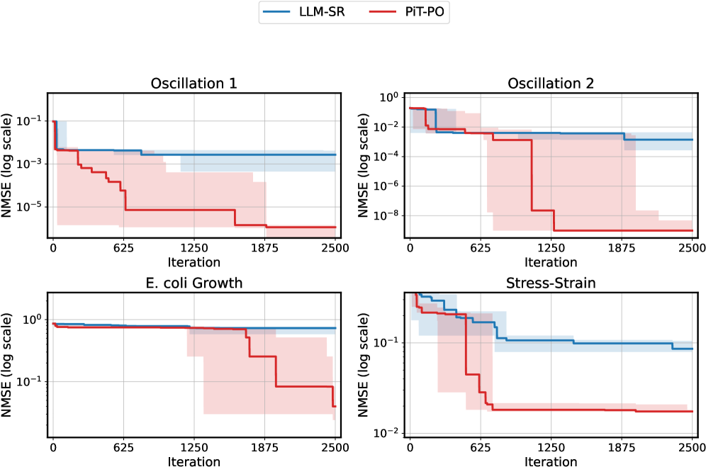
The image presents four separate line charts, each depicting the Normalized Mean Squared Error (NMSE) on a logarithmic scale against the number of iterations. Two models, "LLM-SR" (represented by a blue line) and "PIT-PO" (represented by a red line), are compared across four different scenarios: Oscillation 1, Oscillation 2, E. coli Growth, and Stress-Strain. Shaded regions around each line indicate the standard deviation or confidence interval.
### Components/Axes
* **X-axis:** Iteration, ranging from 0 to 2500.
* **Y-axis:** NMSE (log scale). The scale varies for each chart, but generally spans several orders of magnitude.
* **Legend:** Located at the top-right of the image, it identifies the lines:
* LLM-SR (Blue)
* PIT-PO (Red)
* **Chart Titles:** Each subplot has a title indicating the scenario:
* Oscillation 1 (Top-Left)
* Oscillation 2 (Top-Right)
* E. coli Growth (Bottom-Left)
* Stress-Strain (Bottom-Right)
* **Gridlines:** Present in all charts to aid in reading values.
### Detailed Analysis or Content Details
**Oscillation 1 (Top-Left):**
* Both lines start at approximately 10^-1.
* The blue line (LLM-SR) shows a consistent downward trend, decreasing to approximately 10^-5 by iteration 2500.
* The red line (PIT-PO) also decreases, but more erratically, ending at approximately 10^-3 by iteration 2500.
* The shaded region around the blue line is relatively narrow, indicating lower variance. The red line's shaded region is wider, suggesting higher variance.
**Oscillation 2 (Top-Right):**
* Both lines start around 10^-2.
* The blue line (LLM-SR) initially decreases, then plateaus around 10^-5.
* The red line (PIT-PO) fluctuates around 10^-2, with some dips and rises.
* The shaded regions are relatively narrow for both lines.
**E. coli Growth (Bottom-Left):**
* Both lines start around 10^0.
* The blue line (LLM-SR) decreases in steps, reaching approximately 10^-1 by iteration 2500.
* The red line (PIT-PO) decreases more rapidly and in larger steps, reaching approximately 10^-2 by iteration 2500.
* The shaded regions are wider, indicating higher variance.
**Stress-Strain (Bottom-Right):**
* Both lines start around 10^-1.
* The blue line (LLM-SR) decreases gradually to approximately 10^-2.
* The red line (PIT-PO) initially decreases, then increases sharply around iteration 1250, reaching approximately 10^-1 before decreasing again to approximately 10^-2.
* The shaded regions are relatively narrow for the blue line, but wider for the red line, especially during the increase around iteration 1250.
### Key Observations
* LLM-SR generally exhibits smoother and more consistent decreases in NMSE compared to PIT-PO.
* PIT-PO shows more variability and, in the Stress-Strain scenario, a notable increase in NMSE at iteration 1250.
* The E. coli Growth scenario shows the most significant reduction in NMSE for both models.
* The logarithmic scale emphasizes the relative changes in NMSE, making it easier to compare performance across different scenarios.
### Interpretation
The charts compare the performance of two models, LLM-SR and PIT-PO, in terms of their ability to minimize the Normalized Mean Squared Error (NMSE) across four different dynamic systems. The consistent downward trend of LLM-SR in most scenarios suggests it is more stable and reliable in reducing error. The fluctuations and occasional increases in NMSE for PIT-PO indicate it may be more sensitive to the specific dynamics of the system or require more careful tuning.
The E. coli Growth scenario shows the largest error reduction, potentially indicating that the models are well-suited for modeling biological systems. The Stress-Strain scenario, with PIT-PO's increase in NMSE, suggests a potential instability or limitation of that model under certain conditions. The shaded regions around the lines represent the uncertainty or variance in the model's performance, providing a measure of confidence in the results.
The use of a logarithmic scale is crucial for visualizing the wide range of NMSE values, allowing for a clear comparison of performance even when errors are very small. The charts collectively demonstrate the importance of model selection and parameter tuning for achieving optimal performance in different dynamic systems.