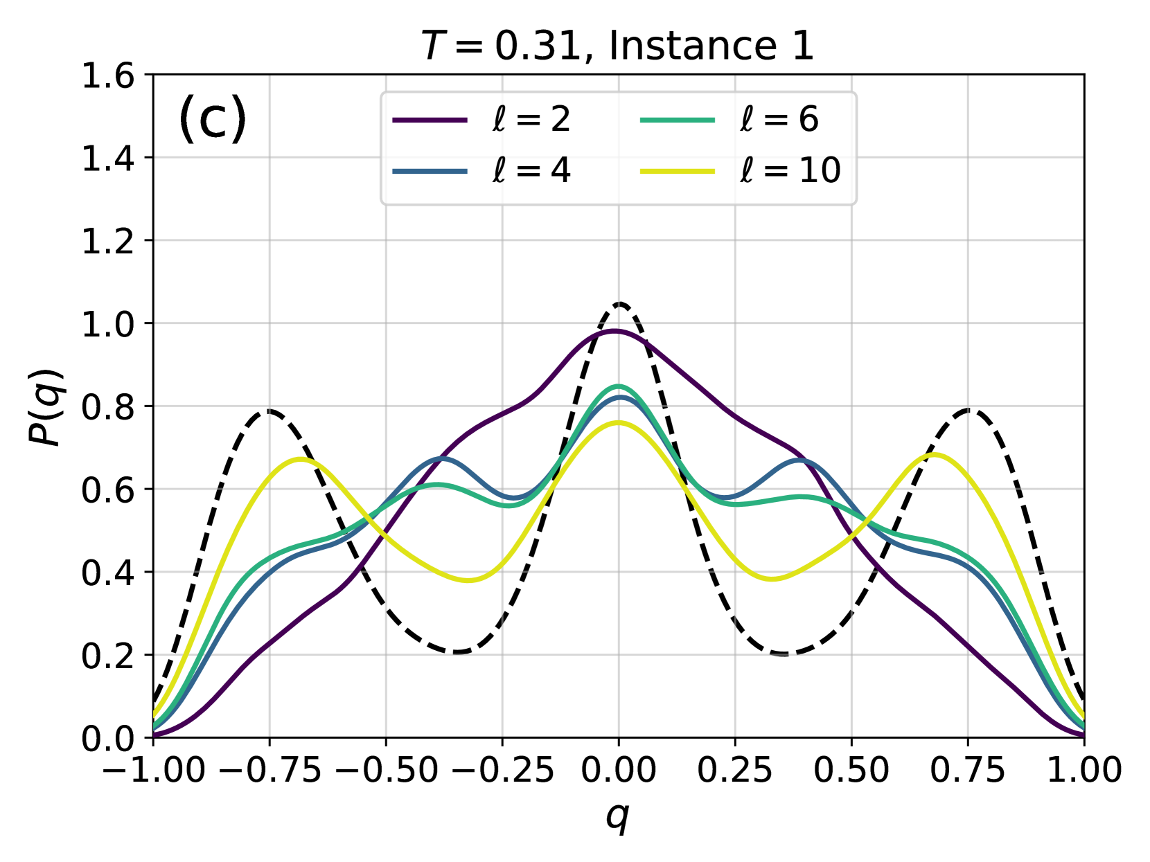
\n ## Line Chart: Probability Distribution of q for Different l Values ### Overview This image presents a line chart illustrating the probability distribution of a variable 'q' for different values of 'l' (2, 4, 6, and 10) under a fixed parameter 'T' of 0.31, for Instance 1. The chart displays the probability density, P(q), as a function of q, ranging from -1.00 to 1.00. The lines are plotted with varying styles (solid, dashed) and colors to distinguish between the different 'l' values. ### Components/Axes * **Title:** T = 0.31, Instance 1 (located at the top-right) * **X-axis Label:** q (located at the bottom-center) * Scale: -1.00 to 1.00, with markers at -1.00, -0.75, -0.50, -0.25, 0.00, 0.25, 0.50, 0.75, 1.00 * **Y-axis Label:** P(q) (located at the left-center) * Scale: 0.0 to 1.6, with gridlines at 0.2 intervals. * **Legend:** Located at the top-right, identifying each line by its 'l' value and color. * l = 2 (Purple, solid line) * l = 4 (Blue, solid line) * l = 6 (Teal, solid line) * l = 10 (Yellow, solid line) * Dashed black line: appears to be a reference or average. ### Detailed Analysis The chart shows four distinct probability distributions, each corresponding to a different value of 'l'. A dashed black line is also present, potentially representing an average or baseline. * **l = 2 (Purple):** The line starts at approximately P(q) = 0.0 at q = -1.00, rises to a peak of approximately P(q) = 0.75 at q = -0.25, then declines to approximately P(q) = 0.0 at q = 1.00. The distribution is relatively narrow and centered around q = -0.25. * **l = 4 (Blue):** The line starts at approximately P(q) = 0.0 at q = -1.00, rises to a peak of approximately P(q) = 0.85 at q = 0.00, then declines to approximately P(q) = 0.0 at q = 1.00. The distribution is centered around q = 0.00. * **l = 6 (Teal):** The line starts at approximately P(q) = 0.0 at q = -1.00, rises to a peak of approximately P(q) = 0.90 at q = 0.25, then declines to approximately P(q) = 0.0 at q = 1.00. The distribution is centered around q = 0.25. * **l = 10 (Yellow):** The line starts at approximately P(q) = 0.0 at q = -1.00, rises to a peak of approximately P(q) = 0.70 at q = 0.50, then declines to approximately P(q) = 0.0 at q = 1.00. The distribution is centered around q = 0.50. * **Dashed Black Line:** This line starts at approximately P(q) = 0.0 at q = -1.00, rises to a peak of approximately P(q) = 0.80 at q = 0.00, then declines to approximately P(q) = 0.0 at q = 1.00. The distributions appear to shift towards positive 'q' values as 'l' increases. ### Key Observations * The distributions are generally unimodal (single peak). * The peak of the distribution shifts to the right (positive q values) as 'l' increases. * The dashed black line appears to represent a central tendency or average of the distributions. * The distributions are not symmetrical. ### Interpretation The chart demonstrates how the probability distribution of 'q' changes with varying values of 'l' under a fixed 'T' value. The shift in the peak of the distribution suggests that as 'l' increases, the most probable value of 'q' also increases. This could indicate a relationship between 'l' and 'q', where higher 'l' values are associated with higher 'q' values. The dashed black line might represent the distribution for a specific 'l' value or an average distribution across different 'l' values. The data suggests a systematic change in the distribution of 'q' as 'l' varies, potentially indicating a parameter influencing the central tendency of the variable. The fact that the distributions are not symmetrical suggests that the underlying process generating 'q' is not symmetrical. Further analysis would be needed to understand the specific meaning of 'l', 'q', and 'T' within the context of the problem being studied.