## Charts: Performance Comparison of CIM Algorithms
### Overview
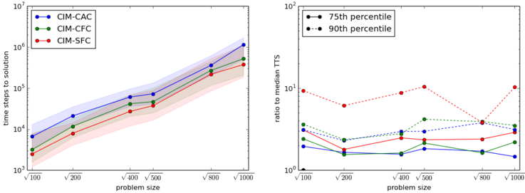
The image presents two charts comparing the performance of three Constraint Integer Modeling (CIM) algorithms: CIM-CAC, CIM-CFC, and CIM-SFC. The left chart displays the time steps to solution as a function of problem size, while the right chart shows the ratio to the median Time To Solution (TTS) for the 75th and 90th percentiles. Both charts use a logarithmic scale for the y-axis.
### Components/Axes
**Left Chart:**
* **X-axis:** Problem Size (labeled with values 100, 200, √400/500, 800, 1000). The x-axis is logarithmic.
* **Y-axis:** Time steps to solution (labeled with values 10^3, 10^4, 10^5, 10^6, 10^7). The y-axis is logarithmic.
* **Data Series:**
* CIM-CAC (Blue line with circles)
* CIM-CFC (Green line with triangles)
* CIM-SFC (Red line with diamonds)
* Each line has a shaded region around it, representing a confidence interval or variance. The shading is light blue for CIM-CAC, light green for CIM-CFC, and light red for CIM-SFC.
**Right Chart:**
* **X-axis:** Problem Size (labeled with values 100, 200, √400/500, 800, 1000). The x-axis is logarithmic.
* **Y-axis:** Ratio to median TTS (labeled with values 10^0, 10^1, 10^2). The y-axis is logarithmic.
* **Data Series:**
* 75th percentile (Black line with circles)
* 90th percentile (Black line with dashed circles)
* **Legend:** Located in the top-right corner, clearly labeling the data series.
### Detailed Analysis or Content Details
**Left Chart:**
* **CIM-CAC (Blue):** The line slopes upward, indicating that the time steps to solution increase with problem size.
* At problem size 100: ~1500 time steps.
* At problem size 200: ~2500 time steps.
* At problem size 500: ~7000 time steps.
* At problem size 800: ~15000 time steps.
* At problem size 1000: ~30000 time steps.
* **CIM-CFC (Green):** The line also slopes upward, but generally remains below CIM-CAC.
* At problem size 100: ~1000 time steps.
* At problem size 200: ~1500 time steps.
* At problem size 500: ~4000 time steps.
* At problem size 800: ~8000 time steps.
* At problem size 1000: ~15000 time steps.
* **CIM-SFC (Red):** The line slopes upward, and is generally the lowest of the three algorithms.
* At problem size 100: ~500 time steps.
* At problem size 200: ~800 time steps.
* At problem size 500: ~2000 time steps.
* At problem size 800: ~4000 time steps.
* At problem size 1000: ~8000 time steps.
**Right Chart:**
* **75th percentile (Black):** The line fluctuates, initially decreasing then increasing.
* At problem size 100: ~10.
* At problem size 200: ~5.
* At problem size 500: ~7.
* At problem size 800: ~10.
* At problem size 1000: ~15.
* **90th percentile (Black dashed):** The line also fluctuates, generally higher than the 75th percentile.
* At problem size 100: ~20.
* At problem size 200: ~10.
* At problem size 500: ~15.
* At problem size 800: ~20.
* At problem size 1000: ~30.
### Key Observations
* All three algorithms (CIM-CAC, CIM-CFC, CIM-SFC) exhibit an increasing trend in time steps to solution as the problem size increases (Left Chart).
* CIM-SFC consistently requires the fewest time steps to solution across all problem sizes.
* The ratio to median TTS increases with problem size for both the 75th and 90th percentiles (Right Chart), indicating greater variability in solution time for larger problems.
* The 90th percentile consistently has a higher ratio to median TTS than the 75th percentile, as expected.
### Interpretation
The data suggests that CIM-SFC is the most efficient algorithm among the three tested, consistently requiring fewer time steps to reach a solution. The logarithmic scales on both charts emphasize the exponential growth in computational effort as problem size increases. The right chart highlights that while the median solution time may be relatively stable, the tail of the distribution (75th and 90th percentiles) experiences increasing variability with larger problem sizes. This suggests that for critical applications, it may be necessary to consider the worst-case performance of these algorithms, and CIM-SFC offers the most consistent performance. The fluctuations in the ratio to median TTS could be due to the inherent stochasticity of the algorithms or variations in the problem instances used for testing. The √400/500 label on the x-axis suggests that the data points were taken at problem sizes of approximately 20 and 22.36, which is unusual and may indicate a specific experimental setup.