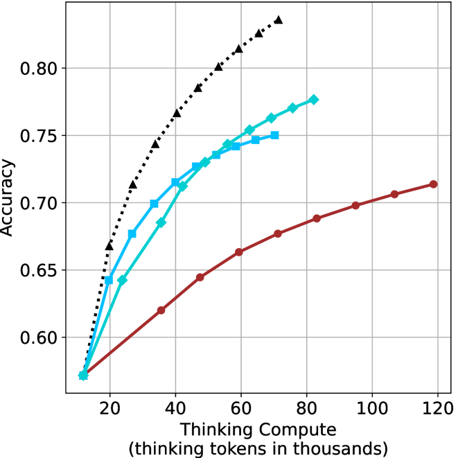
## Line Chart: Accuracy vs. Thinking Compute ### Overview This chart illustrates the relationship between "Thinking Compute" (measured in thousands of thinking tokens) and model "Accuracy." It displays four distinct data series, each representing a different configuration or model variant. All series originate from a common starting point and exhibit diminishing returns as compute increases. ### Components/Axes * **X-Axis:** "Thinking Compute (thinking tokens in thousands)". The scale ranges from 20 to 120, with grid lines at intervals of 20. The data series actually begin at approximately 12,000 tokens. * **Y-Axis:** "Accuracy". The scale ranges from 0.60 to 0.80+, with grid lines at intervals of 0.05. * **Data Series (Legend inferred from visual markers):** * **Black Dotted Line (Triangle markers):** The most efficient series, showing the steepest accuracy gain. * **Cyan Line (Diamond markers):** The second most efficient series. * **Cyan Line (Square markers):** The third most efficient series, closely tracking the diamond-marked line. * **Dark Red/Maroon Line (Circle markers):** The least efficient series, showing the shallowest slope but extending to the highest compute values. ### Detailed Analysis All four data series originate at approximately **(12, 0.57)**. * **Black Dotted Line (Triangles):** * **Trend:** Steepest upward trajectory. * **Data Points (Approximate):** Starts at (12, 0.57), reaches (20, 0.67), (30, 0.71), (40, 0.74), (50, 0.77), (60, 0.80), and terminates at (70, 0.83). * **Cyan Line (Diamonds):** * **Trend:** Strong upward trajectory, second only to the black line. * **Data Points (Approximate):** Starts at (12, 0.57), reaches (25, 0.64), (35, 0.68), (45, 0.71), (55, 0.74), (65, 0.76), (75, 0.77), and terminates at (82, 0.78). * **Cyan Line (Squares):** * **Trend:** Upward trajectory, slightly less efficient than the diamond-marked line. * **Data Points (Approximate):** Starts at (12, 0.57), reaches (20, 0.64), (28, 0.68), (35, 0.70), (45, 0.72), (55, 0.735), (65, 0.745), and terminates at (70, 0.75). * **Dark Red/Maroon Line (Circles):** * **Trend:** Shallowest upward trajectory, indicating lower accuracy gains per unit of compute. * **Data Points (Approximate):** Starts at (12, 0.57), reaches (35, 0.62), (48, 0.645), (60, 0.665), (72, 0.675), (85, 0.69), (95, 0.70), (107, 0.705), and terminates at (120, 0.715). ### Key Observations * **Diminishing Returns:** Every curve exhibits a concave shape, meaning that as "Thinking Compute" increases, the marginal gain in "Accuracy" decreases. * **Efficiency Gap:** There is a significant performance gap between the different series. For example, at 60k tokens, the Black series achieves ~0.80 accuracy, while the Red series achieves only ~0.66. * **Compute Range:** The Black and Square-Cyan series stop at 70k tokens, while the Diamond-Cyan series stops at 82k, and the Red series continues to 120k tokens, suggesting different constraints or limits for each configuration. ### Interpretation This chart likely represents a **test-time compute scaling experiment** for an AI model (such as a reasoning-focused LLM). * **The "Thinking" Paradigm:** The data demonstrates that allowing a model to "think" longer (consume more tokens) improves accuracy, but with clear diminishing returns. * **Model/Strategy Differences:** The four lines likely represent different model sizes or different inference-time search strategies (e.g., different chain-of-thought lengths or search depths). * **Strategic Trade-offs:** The Black line represents the most "efficient" configuration—it achieves the highest accuracy with the least amount of compute. The Red line represents a configuration that is less efficient per token but is capable of scaling to much higher compute levels, perhaps representing a larger model or a more exhaustive search strategy that is computationally expensive but eventually reaches a higher absolute accuracy than it would at lower compute levels. * **Conclusion:** The data suggests that for optimal performance, one should prioritize the configuration represented by the Black line, as it reaches higher accuracy thresholds significantly faster than the other configurations.