## Density Plot Comparison: Sum of Existence Weights for Different k_train Values
### Overview
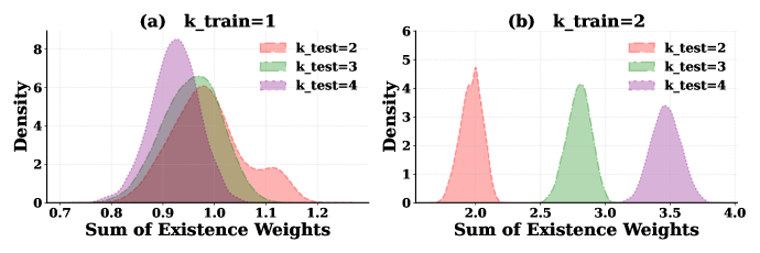
The image displays two side-by-side density plots, labeled (a) and (b), comparing the distribution of the "Sum of Existence Weights" for different values of a parameter `k_train`. Each plot contains three overlaid density curves corresponding to different `k_test` values. The plots illustrate how the distribution of the summed weights changes based on the combination of `k_train` and `k_test`.
### Components/Axes
* **Overall Structure:** Two subplots arranged horizontally.
* **Subplot (a) Title:** `(a) k_train=1`
* **Subplot (b) Title:** `(b) k_train=2`
* **X-Axis (Both Plots):** Label: `Sum of Existence Weights`.
* Plot (a) Range: Approximately 0.7 to 1.2. Major ticks at 0.7, 0.8, 0.9, 1.0, 1.1, 1.2.
* Plot (b) Range: Approximately 1.5 to 4.0. Major ticks at 1.5, 2.0, 2.5, 3.0, 3.5, 4.0.
* **Y-Axis (Both Plots):** Label: `Density`.
* Plot (a) Range: 0 to 8. Major ticks at 0, 2, 4, 6, 8.
* Plot (b) Range: 0 to 6. Major ticks at 0, 2, 4, 6.
* **Legend (Both Plots):** Located in the top-right corner of each subplot. Contains three entries with colored boxes and text labels:
* `k_test=2` (Red/Salmon color)
* `k_test=3` (Green color)
* `k_test=4` (Purple/Lavender color)
### Detailed Analysis
**Subplot (a): k_train=1**
* **Trend Verification:** All three distributions are unimodal and overlap significantly. The distributions for higher `k_test` values are shifted slightly to the left (lower "Sum of Existence Weights") compared to lower `k_test` values.
* **Data Points & Distributions:**
* **k_test=2 (Red):** Peak density is approximately 6.5, occurring at an x-value of ~1.0. The distribution spans roughly from 0.8 to 1.2.
* **k_test=3 (Green):** Peak density is approximately 7.0, occurring at an x-value of ~0.95. The distribution spans roughly from 0.8 to 1.15.
* **k_test=4 (Purple):** Peak density is the highest, approximately 8.0, occurring at an x-value of ~0.9. The distribution spans roughly from 0.75 to 1.1.
* **Key Observation:** The distributions are tightly clustered and overlapping, with peaks between 0.9 and 1.0. The variance appears relatively similar across the three `k_test` values.
**Subplot (b): k_train=2**
* **Trend Verification:** The three distributions are distinct, non-overlapping, and appear as separate, sharp peaks. The peaks shift systematically to the right (higher "Sum of Existence Weights") as `k_test` increases.
* **Data Points & Distributions:**
* **k_test=2 (Red):** Forms a sharp peak. Peak density is approximately 4.8, occurring at an x-value of ~2.0. The distribution is narrow, spanning roughly from 1.7 to 2.3.
* **k_test=3 (Green):** Forms a sharp peak. Peak density is approximately 4.2, occurring at an x-value of ~2.8. The distribution is narrow, spanning roughly from 2.5 to 3.1.
* **k_test=4 (Purple):** Forms a sharp peak. Peak density is approximately 3.5, occurring at an x-value of ~3.5. The distribution is narrow, spanning roughly from 3.2 to 3.8.
* **Key Observation:** The distributions are completely separated. The mean (peak location) of the "Sum of Existence Weights" increases approximately linearly with `k_test`. The peak density decreases slightly as `k_test` increases.
### Key Observations
1. **Effect of k_train:** The value of `k_train` dramatically changes the relationship between `k_test` and the "Sum of Existence Weights".
* For `k_train=1`, the sum is concentrated around 1.0 regardless of `k_test`, with only minor shifts.
* For `k_train=2`, the sum is directly and strongly proportional to `k_test`, resulting in distinct, separated distributions.
2. **Distribution Shape:** For `k_train=1`, the distributions are broader and overlapping. For `k_train=2`, the distributions are much narrower (lower variance) and isolated.
3. **Peak Density:** The maximum density value is highest for `k_train=1, k_test=4` (~8.0) and lowest for `k_train=2, k_test=4` (~3.5).
### Interpretation
This figure demonstrates a fundamental interaction between the parameters `k_train` and `k_test` on the resulting "Sum of Existence Weights."
* **Underlying Mechanism:** The data suggests that `k_train` controls the **scale and separability** of the output. When `k_train=1`, the system's output (the sum) is normalized or constrained to a narrow range near 1.0, making it insensitive to changes in `k_test`. When `k_train=2`, the output becomes sensitive and proportional to `k_test`, suggesting a multiplicative or additive relationship is activated.
* **Implication for a Technical System:** This pattern is characteristic of systems with a **normalization or gating mechanism**. `k_train=1` might represent a state where outputs are normalized (e.g., by a softmax function), collapsing differences. `k_train=2` might represent a state where this normalization is relaxed or altered, allowing the intrinsic differences driven by `k_test` to manifest clearly in the output sum.
* **Notable Anomaly/Insight:** The most striking finding is the qualitative shift in behavior between the two plots. It indicates that the parameter `k_train` is not merely a scaling factor but a **switch that changes the functional regime** of the system from one of saturation/normalization (`k_train=1`) to one of linear response (`k_train=2`). This is critical for understanding model behavior and tuning.