# Technical Document Extraction: Anomaly Detection and Root Cause Localization Workflow
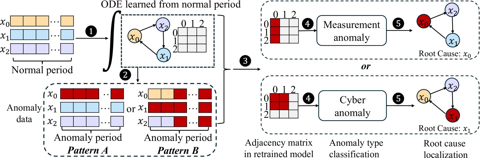
This document describes a technical flow diagram illustrating a process for detecting anomalies, classifying their types, and localizing root causes using Ordinary Differential Equations (ODE) and adjacency matrices.
## 1. Component Isolation
The diagram is organized into a sequential pipeline with five primary stages, indicated by numbered black circles (1 through 5).
### Region A: Input Data (Normal Period)
* **Labels:** $x_0, x_1, x_2$ (representing three distinct variables or sensors).
* **Visual Representation:** Three horizontal time-series bars.
* $x_0$: Yellow/Orange blocks.
* $x_1$: Light Blue blocks.
* $x_2$: Light Purple blocks.
* **Caption:** "Normal period".
### Region B: Model Learning (ODE)
* **Header Text:** "ODE learned from normal period".
* **Process (1):** An arrow leads from the Normal Period data into a large integral symbol ($\int$), representing the learning of an ODE model.
* **Internal Components:**
* **Directed Graph:** Shows relationships between variables. $x_0 \rightarrow x_2$, $x_2 \rightarrow x_1$, and $x_1 \rightarrow x_0$.
* **Adjacency Matrix:** A $3 \times 3$ grid (labeled 0, 1, 2 on both axes). In this "normal" state, the grid cells are empty/white, representing the baseline learned structure.
### Region C: Anomaly Data Patterns
* **Process (2):** An arrow leads from the learned model to the anomaly data section.
* **Label:** "Anomaly data".
* **Pattern A:**
* $x_0$: Red blocks (indicating anomaly).
* $x_1, x_2$: Normal colored blocks (Light Blue/Purple).
* **Caption:** "Anomaly period Pattern A".
* **Pattern B:**
* $x_0, x_1, x_2$: All show a transition from normal colors to Red blocks.
* **Caption:** "Anomaly period Pattern B".
### Region D: Anomaly Classification and Localization
* **Process (3):** A bracket groups the learned model and anomaly data, feeding into two possible branching paths ("or").
* **Footer Labels (Columns):**
1. "Adjacency matrix in retrained model"
2. "Anomaly type classification"
3. "Root cause localization"
#### Path 1: Measurement Anomaly
* **Process (4):** Retrained Adjacency Matrix.
* **Matrix State:** Column 0 is highlighted in **Red**. Columns 1 and 2 are white.
* **Classification:** A rounded box labeled "**Measurement anomaly**".
* **Process (5):** Root Cause Localization.
* **Graph State:** Node $x_0$ is colored **Red**. Nodes $x_1$ and $x_2$ remain normal colors.
* **Text:** "Root Cause: $x_0$".
#### Path 2: Cyber Anomaly
* **Process (4):** Retrained Adjacency Matrix.
* **Matrix State:** Row 0 and Column 0 (specifically the intersection and adjacent cells $(0,0), (0,1), (1,0)$) are highlighted in **Red**.
* **Classification:** A rounded box labeled "**Cyber anomaly**".
* **Process (5):** Root Cause Localization.
* **Graph State:** Node $x_1$ is colored **Red**. Nodes $x_0$ and $x_2$ remain normal colors.
* **Text:** "Root Cause: $x_1$".
---
## 2. Data Table: Adjacency Matrix States
The following table reconstructs the visual state of the $3 \times 3$ matrices during different phases:
| Phase | Cell (0,0) | Cell (0,1) | Cell (0,2) | Cell (1,0) | Cell (1,1) | Cell (1,2) | Cell (2,0) | Cell (2,1) | Cell (2,2) |
| :--- | :--- | :--- | :--- | :--- | :--- | :--- | :--- | :--- | :--- |
| **Normal Period** | White | White | White | White | White | White | White | White | White |
| **Measurement Anomaly** | **Red** | White | White | **Red** | White | White | **Red** | White | White |
| **Cyber Anomaly** | **Red** | **Red** | White | **Red** | White | White | White | White | White |
---
## 3. Logic and Trend Summary
1. **Learning Phase:** The system establishes a baseline (ODE) and a dependency graph ($x_0 \to x_2 \to x_1 \to x_0$) from normal data.
2. **Detection Phase:** When "Anomaly data" is introduced (Pattern A or B), the model is retrained.
3. **Classification Logic:**
* If the retraining results in a **vertical anomaly** in the adjacency matrix (Column 0), it is classified as a **Measurement anomaly**, pointing to $x_0$ as the root cause.
* If the retraining results in an **L-shaped anomaly** in the adjacency matrix (Row 0/Column 0 intersection), it is classified as a **Cyber anomaly**, pointing to $x_1$ as the root cause.
4. **Localization:** The final output identifies the specific node ($x_0$ or $x_1$) responsible for the system deviation.