## Violin Plot: Residual ΔH40 per Dimension
### Overview
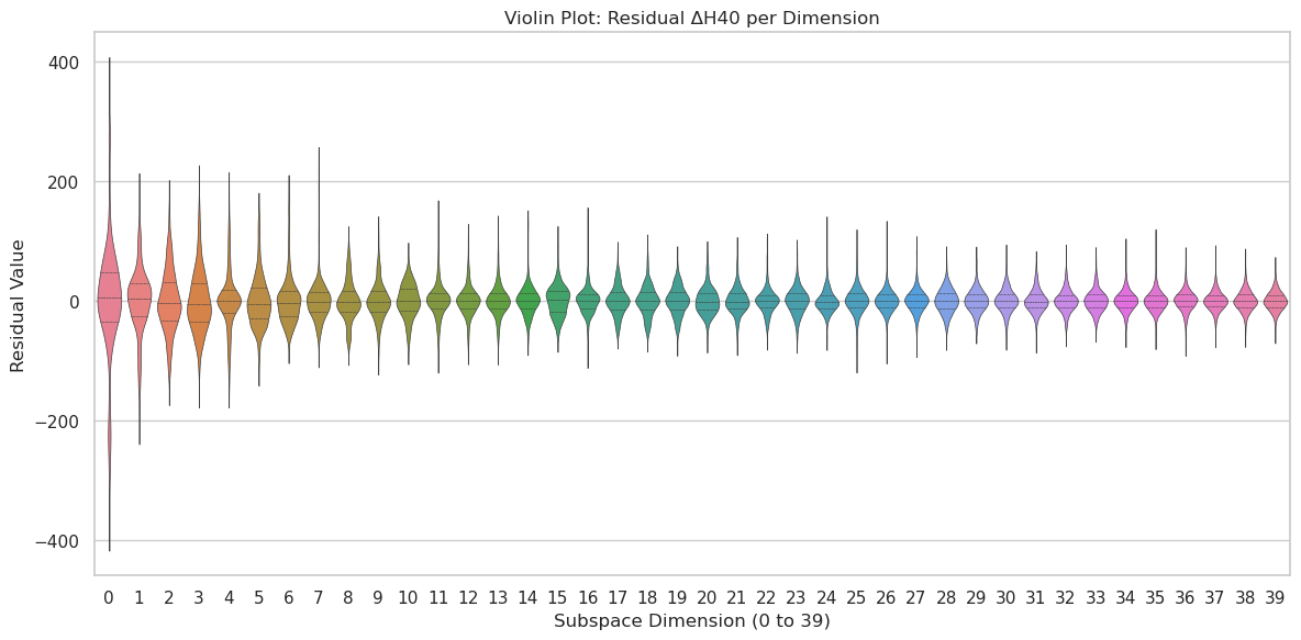
The image displays a violin plot titled "Violin Plot: Residual ΔH40 per Dimension." It visualizes the distribution of residual values (ΔH40) across 40 distinct subspace dimensions, indexed from 0 to 39. Each "violin" represents the probability density of the residual data for a specific dimension, with the width of the violin indicating the frequency of data points at that value.
### Components/Axes
* **Title:** "Violin Plot: Residual ΔH40 per Dimension" (centered at the top).
* **X-Axis:**
* **Label:** "Subspace Dimension (0 to 39)" (centered below the axis).
* **Markers/Ticks:** Integers from 0 to 39, inclusive, spaced evenly. Each number corresponds to the center of a violin.
* **Y-Axis:**
* **Label:** "Residual Value" (rotated 90 degrees, positioned to the left).
* **Scale:** Linear scale.
* **Major Tick Marks:** At -400, -200, 0, 200, and 400.
* **Data Series (Violins):**
* There are 40 individual violin plots, one for each dimension (0-39).
* **Color Scheme:** The violins follow a continuous color gradient. Starting from the left (Dimension 0), the colors progress from a pinkish-red, through orange, yellow, green, teal, blue, and finally to purple/magenta on the right (Dimension 39). This gradient appears to be purely aesthetic for visual distinction and does not represent a separate categorical variable.
* **Legend:** There is no separate legend box. The color-to-dimension mapping is direct and positional along the x-axis.
### Detailed Analysis
* **General Trend:** There is a clear and consistent trend in the shape and spread of the distributions as the subspace dimension increases.
* **Dimensions 0-5 (Leftmost):** These violins are the widest and have the longest vertical tails. Dimension 0 shows the most extreme spread, with its tail extending from approximately -400 to +400. The bulk of the data (the widest part of the violin) is centered near 0 but has significant density extending to ±200.
* **Dimensions 6-20 (Middle-Left):** The violins gradually become narrower and their tails shorten. The central bulge remains around 0, but the overall range of residuals contracts. For example, by Dimension 10, the tails extend roughly from -150 to +150.
* **Dimensions 21-39 (Middle-Right to Rightmost):** The trend of compression continues. The violins become increasingly slender and "pinched," indicating that the residual values are tightly clustered around zero. The vertical extent (range) of the residuals diminishes steadily. By Dimension 39, the violin is very narrow, with most data points appearing to fall within a range of approximately -50 to +50.
* **Central Tendency:** For all dimensions, the median and mode of the residual distribution appear to be centered at or very near 0. There is no visible systematic bias (shift away from zero) across dimensions.
* **Symmetry:** The distributions are largely symmetric around zero for most dimensions, though the early dimensions (0-3) show slight asymmetry with potentially longer tails in the negative direction.
### Key Observations
1. **Monotonic Decrease in Variance:** The most prominent pattern is the monotonic decrease in the variance (spread) of the residual ΔH40 values as the subspace dimension index increases.
2. **High Initial Uncertainty:** The first few dimensions (especially 0) exhibit very high uncertainty or error in the ΔH40 metric, as shown by the large spread of residuals.
3. **Convergence to Precision:** By the final dimensions (35-39), the residuals are highly concentrated near zero, suggesting high precision or consistency in the ΔH40 measurement for these subspaces.
4. **No Obvious Outliers in Trend:** The progression from wide to narrow violins is smooth and consistent. No single dimension breaks the overall trend by having a suddenly wider distribution than its neighbors.
### Interpretation
This plot likely analyzes the performance or stability of a model or measurement (related to "ΔH40") across different components or features of a system, represented by the 40 subspace dimensions.
* **What the Data Suggests:** The data strongly suggests that the reliability or predictability of the ΔH40 metric is highly dependent on the subspace dimension. Lower-order dimensions (0, 1, 2...) are associated with high variability and uncertainty in the residual error. In contrast, higher-order dimensions (30+) yield residuals that are consistently very small.
* **Relationship Between Elements:** The x-axis (Dimension) is the independent variable, and the y-axis (Residual Value) is the dependent variable. The violin shape for each dimension is a direct function of the data's distribution at that x-value. The color gradient, while not carrying quantitative information, helps visually track the progression along the x-axis.
* **Potential Meaning:** In contexts like machine learning (e.g., analyzing latent space dimensions), signal processing, or physical modeling, this pattern could indicate:
* **Feature Importance:** The first few dimensions capture the most significant, but also most volatile, factors influencing ΔH40.
* **Model Convergence:** The model's predictions (or the measurement's consistency) improve dramatically for higher-indexed dimensions.
* **Noise vs. Signal:** Lower dimensions may contain more noise or complex interactions leading to larger residuals, while higher dimensions represent finer, more stable adjustments.
* **Notable Implication:** The key takeaway is that any process or conclusion relying on ΔH40 must account for this dimension-dependent uncertainty. Aggregating residuals across all dimensions without weighting would be misleading, as the error profile is not uniform.