## Diagram & Chart: Knapsack Problem & Time to Solution
### Overview
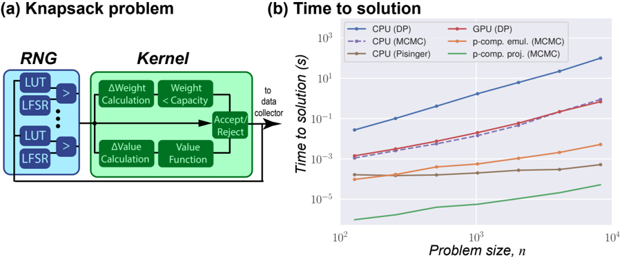
The image presents a diagram illustrating the components of a Knapsack problem solver, alongside a chart showing the time to solution for different algorithms as a function of problem size. The diagram details the Random Number Generator (RNG) and Kernel components, while the chart compares the performance of CPU and GPU implementations using different methods.
### Components/Axes
**Diagram:**
* **Header:** "Knapsack problem"
* **Left Block:** "RNG" containing "LUT" and "LFSR" repeated multiple times. Arrows indicate flow.
* **Right Block:** "Kernel" containing "ΔWeight Calculation", "Weight < Capacity", "Accept/Reject", "ΔValue Calculation", "Value Function". Arrows indicate flow.
* **Connections:** Arrows connect the RNG to the Kernel for both weight and value calculations. An arrow leads from "Accept/Reject" to "to data collector".
**Chart:**
* **Title:** "Time to solution"
* **X-axis:** "Problem size, n" (logarithmic scale, ranging from 10<sup>2</sup> to 10<sup>4</sup>)
* **Y-axis:** "Time to solution (s)" (logarithmic scale, ranging from 10<sup>-5</sup> to 10<sup>1</sup>)
* **Legend (top-right):**
* Blue Solid Line: "CPU (DP)"
* Red Solid Line: "GPU (DP)"
* Orange Dashed Line: "CPU (MCMC)"
* Yellow Dashed Line: "p-comp. emul. (MCMC)"
* Green Solid Line: "CPU (Pisinger)"
* Teal Dashed Line: "p-comp. proj. (MCMC)"
### Detailed Analysis or Content Details
**Diagram:**
The diagram illustrates a system for solving the Knapsack problem. The "RNG" block generates random numbers using Look-Up Tables (LUTs) and Linear Feedback Shift Registers (LFSRs). These random numbers are fed into the "Kernel" block, where weight and value differences are calculated. The calculated weight is compared against the "Capacity". Based on this comparison, solutions are either "Accept"ed or "Reject"ed and sent to a "data collector".
**Chart:**
* **CPU (DP) (Blue Solid Line):** Starts at approximately 0.1 seconds at n=10<sup>2</sup>, increases steadily to approximately 10 seconds at n=10<sup>4</sup>. The line is nearly linear on this log-log scale.
* **GPU (DP) (Red Solid Line):** Starts at approximately 0.01 seconds at n=10<sup>2</sup>, increases to approximately 0.1 seconds at n=10<sup>4</sup>. The line is nearly linear on this log-log scale.
* **CPU (MCMC) (Orange Dashed Line):** Starts at approximately 0.001 seconds at n=10<sup>2</sup>, increases to approximately 0.01 seconds at n=10<sup>4</sup>. The line is relatively flat.
* **p-comp. emul. (MCMC) (Yellow Dashed Line):** Starts at approximately 0.0005 seconds at n=10<sup>2</sup>, increases to approximately 0.005 seconds at n=10<sup>4</sup>. The line is relatively flat.
* **CPU (Pisinger) (Green Solid Line):** Starts at approximately 0.00001 seconds at n=10<sup>2</sup>, increases to approximately 0.0001 seconds at n=10<sup>4</sup>. The line is nearly flat.
* **p-comp. proj. (MCMC) (Teal Dashed Line):** Starts at approximately 0.000005 seconds at n=10<sup>2</sup>, increases to approximately 0.00005 seconds at n=10<sup>4</sup>. The line is nearly flat.
### Key Observations
* The CPU (DP) method is significantly slower than all other methods, especially as the problem size increases.
* The GPU (DP) method is faster than the CPU (DP) method, but still slower than the MCMC-based methods.
* The MCMC-based methods (CPU (MCMC), p-comp. emul. (MCMC), CPU (Pisinger), and p-comp. proj. (MCMC)) exhibit relatively constant solution times regardless of problem size.
* The "p-comp. proj. (MCMC)" method is the fastest across all problem sizes.
* The chart uses a logarithmic scale for both axes, indicating a wide range of values.
### Interpretation
The data suggests that for solving the Knapsack problem, Dynamic Programming (DP) is computationally expensive and scales poorly with problem size. The GPU implementation of DP offers some improvement over the CPU implementation, but the performance is still limited. Markov Chain Monte Carlo (MCMC) methods, particularly the "p-comp. proj. (MCMC)" variant, provide a much more efficient solution, with solution times remaining relatively constant even as the problem size increases. This indicates that MCMC methods are better suited for large-scale Knapsack problems.
The diagram illustrates the underlying process of the Knapsack solver, highlighting the role of random number generation and the iterative acceptance/rejection process within the Kernel. The connection between the RNG and the Kernel suggests that the quality of the random numbers is crucial for the performance of the solver. The "Accept/Reject" step implies a probabilistic approach to finding optimal solutions, which is consistent with the use of MCMC methods. The "to data collector" arrow indicates that the accepted solutions are accumulated for analysis.