\n
## Histogram: Sentences per Trace
### Overview
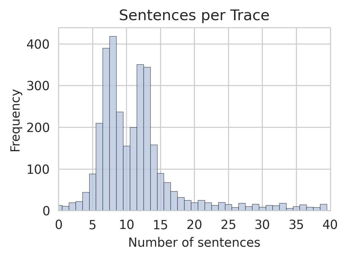
The image displays a histogram titled "Sentences per Trace," illustrating the frequency distribution of the number of sentences contained within individual traces. The chart shows a right-skewed distribution, with the majority of traces containing a relatively low number of sentences, and a long tail extending to higher counts.
### Components/Axes
* **Chart Title:** "Sentences per Trace" (centered at the top).
* **X-Axis:** Labeled "Number of sentences." The scale runs from 0 to 40, with major tick marks at intervals of 5 (0, 5, 10, 15, 20, 25, 30, 35, 40).
* **Y-Axis:** Labeled "Frequency." The scale runs from 0 to over 400, with major tick marks at intervals of 100 (0, 100, 200, 300, 400).
* **Data Series:** A single data series represented by light blue vertical bars. There is no legend, as the chart contains only one category of data.
* **Grid:** A light gray grid is present, with horizontal lines at each major y-axis tick and vertical lines at each major x-axis tick.
### Detailed Analysis
The histogram bins appear to have a width of 1 unit on the x-axis. Below is an approximate reconstruction of the frequency for key bins, based on visual estimation against the y-axis grid. Values are approximate with inherent uncertainty.
* **0-1 sentences:** Very low frequency, approximately 10-20.
* **2-3 sentences:** Frequency rises to approximately 20-30.
* **4-5 sentences:** Frequency increases to approximately 40-50.
* **5-6 sentences:** Sharp increase to approximately 90.
* **6-7 sentences:** Further increase to approximately 210.
* **7-8 sentences:** **Highest peak (mode)**, frequency approximately 420.
* **8-9 sentences:** High frequency, approximately 390.
* **9-10 sentences:** Frequency drops to approximately 240.
* **10-11 sentences:** Frequency approximately 155.
* **11-12 sentences:** **Secondary peak**, frequency approximately 350.
* **12-13 sentences:** High frequency, approximately 345.
* **13-14 sentences:** Frequency drops to approximately 160.
* **14-15 sentences:** Frequency approximately 90.
* **15-16 sentences:** Frequency approximately 70.
* **16-17 sentences:** Frequency approximately 50.
* **17-18 sentences:** Frequency approximately 30.
* **18-20 sentences:** Frequencies taper off, ranging between approximately 15-25.
* **20-40 sentences:** A long, low tail with frequencies generally below 20, showing minor fluctuations but no significant peaks.
### Key Observations
1. **Bimodal Distribution:** The distribution is not a simple bell curve. It has a primary mode at 7-8 sentences and a distinct secondary mode at 12-13 sentences.
2. **Right Skew:** The tail of the distribution extends significantly to the right, indicating that while most traces are short, there is a subset of traces with a much higher sentence count (up to 40).
3. **Concentration:** The vast majority of traces (the bulk of the area under the histogram) contain between 5 and 15 sentences.
4. **Low-End Frequency:** Very few traces contain 0-4 sentences.
### Interpretation
This histogram provides a quantitative profile of trace length within the analyzed dataset. The data suggests that the process or system generating these traces most commonly produces outputs of moderate length, clustering around two typical lengths: one around 7-8 sentences and another around 12-13 sentences. This could indicate two common modes of operation, two types of tasks, or two levels of complexity in the underlying activity being traced.
The long tail to the right is significant. It demonstrates that while uncommon, the system is capable of generating, or occasionally encounters, scenarios that result in much more verbose traces (20-40 sentences). These outliers might represent complex error states, detailed debugging outputs, or unusually lengthy transactions. The relative scarcity of very short traces (0-4 sentences) suggests that the traced activity typically involves a minimum level of substantive interaction or reporting. For a technical document, this distribution is crucial for understanding system behavior, setting expectations for log size, and designing storage or analysis tools that can handle both the common case and the outliers.