## Mathematical Commutative Diagram: Functorial Relationships
### Overview
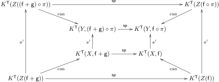
The image displays a commutative diagram from advanced mathematics, likely within category theory, homological algebra, or algebraic topology. It illustrates the relationships between several functorial constructions, denoted by `K^T`, applied to different combinations of objects (`X`, `Y`, `Z`) and morphisms or functions (`f`, `g`). The diagram is structured as a rectangular grid with six nodes connected by directed arrows, each labeled with a specific map or transformation (`sp`, `can`, `π'`).
### Components/Axes
The diagram consists of six nodes arranged in two rows and three columns, with the central column containing two vertically stacked nodes.
**Nodes (from top-left, moving right and down):**
1. **Top-Left:** `K^T(Z((f + g) ∘ π))`
2. **Top-Center:** `K^T(Y, (f + g) ∘ π)`
3. **Top-Right:** `K^T(Z(f ∘ π))`
4. **Bottom-Left:** `K^T(Z(f + g))`
5. **Bottom-Center:** `K^T(X, f + g)`
6. **Bottom-Right:** `K^T(Z(f))`
**Arrows and Labels:**
* **Horizontal Arrows (labeled `sp`):**
* From `K^T(Z((f + g) ∘ π))` to `K^T(Z(f ∘ π))` (Top row, left to right).
* From `K^T(Y, (f + g) ∘ π)` to `K^T(Y, f ∘ π)` (Top-center to a node not explicitly drawn but implied by the arrow's endpoint, which is `K^T(Y, f ∘ π)`).
* From `K^T(X, f + g)` to `K^T(X, f)` (Bottom-center to a node not explicitly drawn but implied by the arrow's endpoint, which is `K^T(X, f)`).
* From `K^T(Z(f + g))` to `K^T(Z(f))` (Bottom row, left to right).
* **Diagonal Arrows (labeled `can`):**
* From `K^T(Z((f + g) ∘ π))` to `K^T(Y, (f + g) ∘ π)` (Top-left to top-center).
* From `K^T(Z(f ∘ π))` to `K^T(Y, f ∘ π)` (Top-right to the implied top-center-right node).
* From `K^T(Z(f + g))` to `K^T(X, f + g)` (Bottom-left to bottom-center).
* From `K^T(Z(f))` to `K^T(X, f)` (Bottom-right to the implied bottom-center-right node).
* **Vertical Arrows (labeled `π'`):**
* From `K^T(Y, (f + g) ∘ π)` to `K^T(X, f + g)` (Top-center to bottom-center).
* From `K^T(Y, f ∘ π)` to `K^T(X, f)` (Implied top-center-right to implied bottom-center-right).
* From `K^T(Z((f + g) ∘ π))` to `K^T(Z(f + g))` (Top-left to bottom-left).
* From `K^T(Z(f ∘ π))` to `K^T(Z(f))` (Top-right to bottom-right).
### Detailed Analysis
The diagram is a network of commutative squares and triangles. The primary structure is a large outer rectangle whose corners are the four `Z`-nodes. Inside this, a smaller rectangle is formed by the `Y` and `X` nodes. The arrows define specific pathways between these constructions.
* **`sp` arrows:** These horizontal arrows likely represent a "specialization" or "splitting" map, transforming a construction involving a sum `(f + g)` into one involving only `f`.
* **`can` arrows:** These diagonal arrows likely represent "canonical" maps, relating constructions on the object `Z` to corresponding constructions on objects `Y` or `X`.
* **`π'` arrows:** These vertical arrows likely represent a map induced by a projection `π`, relating constructions involving `(f + g) ∘ π` or `f ∘ π` to those involving `f + g` or `f` directly.
The diagram asserts that all paths from a given starting node to a given ending node are equivalent. For example, the path from `K^T(Z((f + g) ∘ π))` to `K^T(X, f + g)` can be taken either via `can` then `π'`, or via `π'` then `can`. The commutativity of the diagram is the key mathematical statement.
### Key Observations
1. **Symmetry:** The diagram exhibits a high degree of symmetry. The left half deals with the sum `(f + g)`, while the right half deals with the single function `f`. The top row involves composition with `π`, while the bottom row does not.
2. **Implied Nodes:** Two nodes (`K^T(Y, f ∘ π)` and `K^T(X, f)`) are not explicitly drawn as boxes but are clearly implied as the targets of multiple arrows. This is a common shorthand in such diagrams.
3. **Consistent Labeling:** The labels `sp`, `can`, and `π'` are used consistently for all arrows of the same orientation and type, indicating they represent the same kind of natural transformation or functorial map applied in different contexts.
### Interpretation
This diagram is a formal, visual proof of the compatibility between several natural transformations (`sp`, `can`, `π'`) acting on a functor `K^T`. It demonstrates that the operations of "adding functions" (`f + g`), "composing with a projection" (`∘ π`), and applying the canonical and specialization maps all interact in a coherent, predictable way.
The commutativity ensures that the mathematical structures are well-behaved. For instance, it shows that the process of first specializing a sum of composed functions and then projecting is the same as first projecting the sum and then specializing. Such diagrams are fundamental in areas like derived functors, spectral sequences, or the study of model categories, where tracking how different operations interact is crucial. The diagram encapsulates a complex set of relationships into a single, verifiable geometric statement.