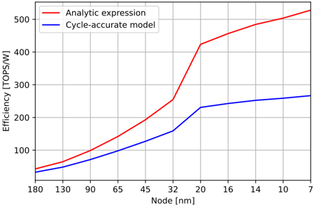
## Line Graph: Efficiency vs. Node Size Comparison ### Overview The image is a line graph comparing the efficiency (in TOPS/W) of two computational models—Analytic expression and Cycle-accurate model—as a function of transistor node size (in nanometers). The graph spans node sizes from 7 nm to 180 nm, with efficiency values ranging from 0 to 500 TOPS/W. --- ### Components/Axes - **X-axis (Horizontal)**: Labeled "Node [nm]" with tick marks at 7, 10, 14, 16, 20, 32, 45, 65, 90, 130, and 180 nm. - **Y-axis (Vertical)**: Labeled "Efficiency [TOPS/W]" with tick marks at 0, 100, 200, 300, 400, and 500. - **Legend**: Located in the top-left corner, with: - **Red line**: "Analytic expression" - **Blue line**: "Cycle-accurate model" --- ### Detailed Analysis #### Analytic Expression (Red Line) - **Trend**: Starts at ~50 TOPS/W at 180 nm, increases gradually until ~32 nm (~250 TOPS/W), then rises sharply to ~520 TOPS/W at 7 nm. - **Key Data Points**: - 180 nm: ~50 TOPS/W - 90 nm: ~100 TOPS/W - 65 nm: ~150 TOPS/W - 45 nm: ~200 TOPS/W - 32 nm: ~250 TOPS/W - 20 nm: ~420 TOPS/W - 10 nm: ~500 TOPS/W - 7 nm: ~520 TOPS/W #### Cycle-Accurate Model (Blue Line) - **Trend**: Starts at ~40 TOPS/W at 180 nm, increases gradually to ~260 TOPS/W at 7 nm. - **Key Data Points**: - 180 nm: ~40 TOPS/W - 90 nm: ~80 TOPS/W - 65 nm: ~110 TOPS/W - 45 nm: ~140 TOPS/W - 32 nm: ~170 TOPS/W - 20 nm: ~220 TOPS/W - 10 nm: ~250 TOPS/W - 7 nm: ~260 TOPS/W --- ### Key Observations 1. **Divergence at Smaller Nodes**: The Analytic expression model predicts significantly higher efficiency gains at smaller nodes (e.g., 7 nm: ~520 TOPS/W vs. ~260 TOPS/W for Cycle-accurate). 2. **Slope Difference**: The red line (Analytic) has a steeper slope, especially between 32 nm and 7 nm, indicating a nonlinear relationship. 3. **Consistent Gap**: The Analytic model consistently outperforms the Cycle-accurate model across all node sizes. --- ### Interpretation - **Model Behavior**: The Analytic expression model assumes idealized efficiency improvements with smaller nodes, while the Cycle-accurate model incorporates real-world constraints (e.g., power leakage, heat dissipation), resulting in more conservative estimates. - **Technical Implications**: The gap between the two models widens at smaller nodes, suggesting that the Analytic model may overestimate efficiency gains in advanced semiconductor designs. This highlights the importance of cycle-accurate simulations for realistic performance predictions. - **Anomaly**: The sharp rise in the Analytic model’s efficiency between 32 nm and 7 nm could indicate an idealized scaling assumption (e.g., ignoring physical limits like quantum tunneling) not captured by the Cycle-accurate model. --- ### Spatial Grounding - **Legend**: Top-left corner, clearly associating colors with models. - **Lines**: Red (Analytic) and blue (Cycle-accurate) are distinct and non-overlapping. - **Axis Labels**: Positioned at the bottom (x-axis) and left (y-axis), with gridlines for reference. --- ### Content Details - **X-axis Range**: 7 nm to 180 nm (logarithmic-like spacing between ticks). - **Y-axis Range**: 0 to 500 TOPS/W (linear scale). - **No Data Table**: Values are inferred from line intersections with gridlines. --- ### Final Notes The graph underscores the trade-off between theoretical (Analytic) and practical (Cycle-accurate) efficiency predictions in semiconductor design. The Cycle-accurate model’s slower growth suggests it accounts for physical limitations, making it more reliable for real-world applications.