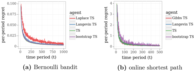
\n ## Charts: Per-Period Regret vs. Time Period for Different Agents ### Overview The image presents two line charts comparing the per-period regret of different agents over time. The left chart (a) depicts results for a "Bernoulli bandit" scenario, while the right chart (b) shows results for an "online shortest path" scenario. Both charts share a similar structure, plotting per-period regret on the y-axis against time period (t) on the x-axis. ### Components/Axes Both charts have the following components: * **X-axis:** Labeled "time period (t)". The scale ranges from 0 to 1000 for chart (a) and 0 to 500 for chart (b). * **Y-axis:** Labeled "per-period regret". Chart (a) ranges from 0 to 0.100, while chart (b) ranges from 0 to 4. * **Legend:** Located in the top-right corner of each chart, labeled "agent". The agents are: * Laplace TS (Red) * Langevin TS (Blue) * TS (Green) * bootstrap TS (Purple) ### Detailed Analysis or Content Details **Chart (a): Bernoulli bandit** * **Laplace TS (Red):** The line starts at approximately 0.08, rapidly decreases to around 0.03 by t=100, and then gradually declines to approximately 0.015 by t=1000. * **Langevin TS (Blue):** The line begins at approximately 0.06, decreases to around 0.02 by t=100, and continues to decline slowly, reaching approximately 0.01 by t=1000. * **TS (Green):** The line starts at approximately 0.05, decreases rapidly to around 0.015 by t=100, and then declines slowly to approximately 0.01 by t=1000. * **bootstrap TS (Purple):** The line begins at approximately 0.06, decreases to around 0.02 by t=100, and then declines slowly, reaching approximately 0.01 by t=1000. **Chart (b): online shortest path** * **Gibbs TS (Red):** The line starts at approximately 3.5, rapidly decreases to around 1.5 by t=100, and then declines slowly to approximately 0.5 by t=500. * **Langevin TS (Blue):** The line begins at approximately 3.0, decreases to around 1.0 by t=100, and then declines slowly, reaching approximately 0.3 by t=500. * **TS (Green):** The line starts at approximately 2.5, decreases rapidly to around 0.7 by t=100, and then declines slowly to approximately 0.2 by t=500. * **bootstrap TS (Purple):** The line begins at approximately 2.5, decreases to around 0.8 by t=100, and then declines slowly, reaching approximately 0.3 by t=500. ### Key Observations * In both charts, all agents exhibit a decreasing trend in per-period regret as time progresses, indicating learning and improvement. * In chart (a), the Laplace TS agent initially has the highest regret, but its regret decreases rapidly. * In chart (b), the Gibbs TS agent initially has the highest regret, but its regret decreases rapidly. * The differences in regret between agents become smaller as time increases in both scenarios. * The scale of the y-axis is significantly different between the two charts, reflecting the different magnitudes of regret in the two scenarios. ### Interpretation The charts demonstrate the performance of different Thompson Sampling (TS) variants in two distinct reinforcement learning environments: a Bernoulli bandit and an online shortest path problem. The per-period regret metric quantifies the cumulative loss incurred by the agent due to suboptimal decisions. The decreasing trend in regret across all agents indicates that they are learning to make better decisions over time. The initial differences in regret likely reflect the varying exploration-exploitation trade-offs and convergence rates of the different TS algorithms. The fact that the regret curves converge as time increases suggests that all agents eventually achieve a similar level of performance. The higher regret values observed in the online shortest path scenario (chart b) compared to the Bernoulli bandit scenario (chart a) may be due to the increased complexity of the shortest path problem, which requires the agent to learn a more complex policy. The choice of algorithm appears to have a more pronounced effect in the online shortest path scenario, as the initial differences in regret are more substantial. The charts provide valuable insights into the effectiveness of different TS algorithms in different reinforcement learning settings. They highlight the importance of considering the specific characteristics of the environment when selecting an algorithm.