## Statistical Distribution Charts: Tensor Value Histograms
### Overview
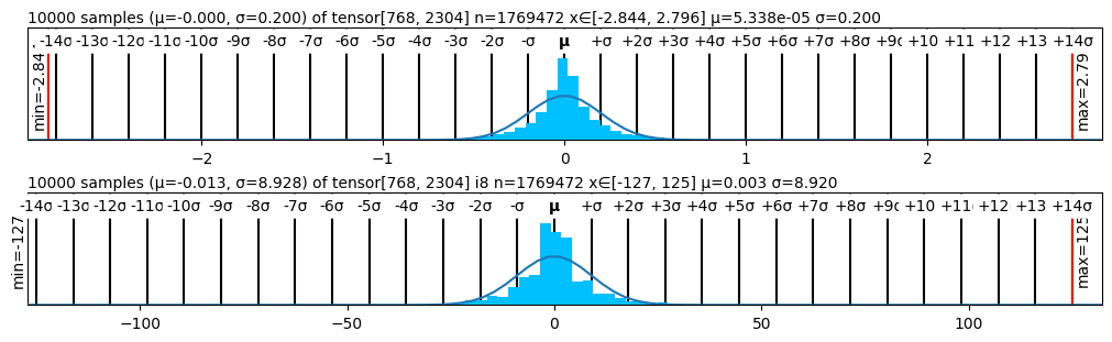
The image displays two vertically stacked statistical plots, each showing a histogram of 10,000 samples drawn from a large tensor (n=1,769,472 elements). Both plots include an overlaid normal distribution curve and detailed statistical annotations. The top plot analyzes a tensor with a very narrow distribution, while the bottom plot analyzes a tensor with a much wider spread.
### Components/Axes
**Top Plot:**
* **Title/Header Text:** `10000 samples (μ=-0.000, σ=0.200) of tensor[768, 2304] n=1769472 x∈[-2.844, 2.796] μ=5.338e-05 σ=0.200`
* **X-Axis:** A dual-scale axis.
* **Upper Scale (in σ units):** Markers from `-14σ` to `+14σ`, with `μ` (mean) at the center.
* **Lower Scale (absolute values):** Major tick marks at `-2`, `-1`, `0`, `1`, `2`.
* **Vertical Reference Lines:**
* A red vertical line on the far left labeled `min=-2.844`.
* A red vertical line on the far right labeled `max=2.796`.
* **Data Series:**
* **Histogram:** Light blue bars representing the frequency distribution of the 10,000 samples.
* **Normal Curve:** A black line representing a theoretical normal (Gaussian) distribution with the given mean (μ) and standard deviation (σ).
**Bottom Plot:**
* **Title/Header Text:** `10000 samples (μ=-0.013, σ=8.928) of tensor[768, 2304] i8 n=1769472 x∈[-127, 125] μ=0.003 σ=8.920`
* **X-Axis:** A dual-scale axis.
* **Upper Scale (in σ units):** Markers from `-14σ` to `+14σ`, with `μ` (mean) at the center.
* **Lower Scale (absolute values):** Major tick marks at `-100`, `-50`, `0`, `50`, `100`.
* **Vertical Reference Lines:**
* A red vertical line on the far left labeled `min=-127`.
* A red vertical line on the far right labeled `max=125`.
* **Data Series:**
* **Histogram:** Light blue bars representing the frequency distribution of the 10,000 samples.
* **Normal Curve:** A black line representing a theoretical normal distribution.
### Detailed Analysis
**Top Plot Analysis:**
* **Trend Verification:** The histogram forms a very sharp, narrow peak centered at 0, closely following the overlaid normal curve. The distribution is highly concentrated.
* **Data Points & Values:**
* Sample Mean (μ): Approximately -0.000 (from sample) or 5.338e-05 (from full tensor).
* Sample Standard Deviation (σ): 0.200.
* Full Tensor Range: [-2.844, 2.796].
* The visual spread of the histogram aligns with the small σ=0.200. The min/max lines are far outside the main data cluster, indicating extreme outliers are rare.
**Bottom Plot Analysis:**
* **Trend Verification:** The histogram forms a broader, bell-shaped peak centered near 0, also following its normal curve. The spread is significantly wider than the top plot.
* **Data Points & Values:**
* Sample Mean (μ): Approximately -0.013 (from sample) or 0.003 (from full tensor).
* Sample Standard Deviation (σ): 8.928 (sample) vs. 8.920 (full tensor).
* Full Tensor Range: [-127, 125]. This range is characteristic of an 8-bit integer (`i8`) data type, as noted in the title.
* The histogram's width corresponds to the larger σ≈8.92. The min/max lines at -127 and 125 are at the theoretical limits of the `i8` range.
### Key Observations
1. **Scale Discrepancy:** The two tensors have vastly different scales. The top tensor's values are confined within ~±3, while the bottom tensor's values span the full 8-bit integer range of ~±127.
2. **Distribution Shape:** Both distributions are approximately normal (Gaussian) and centered near zero, suggesting the data may be normalized or represent residuals/weights with zero mean.
3. **Data Type Indicator:** The bottom plot's title includes "i8", explicitly identifying its data type as signed 8-bit integer, which explains the hard limits at -127 and 125.
4. **Sampling Fidelity:** The sample statistics (μ, σ) are very close to the full tensor statistics in both cases, indicating the 10,000-sample subset is a good representation of the whole.
### Interpretation
These charts are diagnostic tools for understanding the value distribution within two different tensors, likely from a machine learning model (given dimensions like [768, 2304], common in transformer architectures).
* **What the data suggests:** The top tensor contains high-precision, low-magnitude values (possibly floating-point activations or normalized weights). The bottom tensor contains low-precision, high-magnitude values constrained to the `i8` range (possibly quantized weights or integer activations).
* **Relationship between elements:** The plots allow for a direct comparison of the statistical properties (central tendency, spread, outliers) of two different data representations. The use of a shared σ-scale on the upper x-axis facilitates this comparison, showing that both distributions, despite their different absolute scales, follow a similar Gaussian shape relative to their own standard deviations.
* **Notable anomalies:** There are no major anomalies; the data conforms well to the expected normal distributions. The key insight is the stark contrast in scale and data type between the two tensors, which is critical for tasks like model quantization, where understanding value ranges is essential to avoid clipping and maintain accuracy.