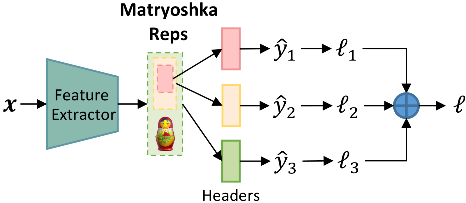
## Diagram: Matryoshka Representation Learning Architecture ### Overview This image is a technical diagram illustrating a machine learning architecture called "Matryoshka Representation Learning." It depicts a data flow from an input `x` through a feature extractor to produce nested representations ("Matryoshka Reps"), which are then processed by multiple parallel "Headers" to generate predictions and individual losses, finally aggregated into a single total loss `ℓ`. The diagram uses a left-to-right flow with color-coded components and a Russian Matryoshka doll icon to symbolize the nested, multi-scale nature of the representations. ### Components/Axes The diagram contains the following labeled components and symbols, listed in order of data flow from left to right: 1. **Input**: Labeled `x` (italicized mathematical symbol). 2. **Feature Extractor**: A teal-colored trapezoid block with the text "Feature Extractor" inside. 3. **Matryoshka Reps**: A central block with the title "Matryoshka Reps" above it. This block contains: * A green dashed-line rectangle. * Inside it, a nested set of three rectangles with dashed borders: a large light orange rectangle, a medium pink rectangle inside that, and a small red rectangle inside the pink one. * A small icon of a traditional Russian Matryoshka doll placed at the bottom of the green dashed rectangle. 4. **Headers**: Three parallel rectangular blocks to the right of the Matryoshka Reps, collectively labeled "Headers" below them. They are color-coded: * **Top Header**: Pink rectangle. * **Middle Header**: Light orange/yellow rectangle. * **Bottom Header**: Green rectangle. 5. **Predictions**: Mathematical symbols for predicted outputs, each connected to a header: * `ŷ₁` (y-hat subscript 1) from the pink header. * `ŷ₂` (y-hat subscript 2) from the light orange header. * `ŷ₃` (y-hat subscript 3) from the green header. 6. **Individual Losses**: Mathematical symbols for loss values, each connected to a prediction: * `ℓ₁` (script l subscript 1) from `ŷ₁`. * `ℓ₂` (script l subscript 2) from `ŷ₂`. * `ℓ₃` (script l subscript 3) from `ŷ₃`. 7. **Aggregation Node**: A blue circle with a plus sign (`+`) inside, located to the right of the individual losses. 8. **Total Loss**: The final output, labeled `ℓ` (script l), connected from the aggregation node. ### Detailed Analysis **Spatial Layout and Flow:** * The flow is strictly left-to-right, indicated by black arrows connecting each component. * The **Matryoshka Reps** block is the central hub. Three arrows originate from its right side, each pointing to one of the three **Headers**. This visually represents that the nested representations are being "unpacked" or accessed at different scales. * The three parallel processing paths (Header -> Prediction -> Loss) are vertically stacked. The **pink path** is top, the **light orange path** is middle, and the **green path** is bottom. * The three individual loss values (`ℓ₁`, `ℓ₂`, `ℓ₃`) are connected by arrows to the central **aggregation node** (blue circle with `+`), indicating they are summed or combined. * The final arrow from the aggregation node points to the total loss `ℓ`. **Component Relationships & Color Coding:** * There is a direct visual correspondence between the nested rectangles inside the **Matryoshka Reps** and the **Headers**: * The innermost **red** rectangle corresponds to the **pink** header (top path). * The middle **pink** rectangle corresponds to the **light orange** header (middle path). * The outermost **light orange** rectangle corresponds to the **green** header (bottom path). * *Note: There is a slight color mismatch between the innermost rectangle (red) and its corresponding header (pink), but the positional and sequential logic is clear.* * This color/position mapping reinforces the core concept: the model produces a single, nested representation from which features of different granularities (small/precise to large/general) can be extracted by different headers. ### Key Observations 1. **Nested Representation Core**: The diagram's central metaphor is the Matryoshka doll, explicitly shown and named. This indicates the model learns a single representation that contains useful sub-representations of varying sizes/dimensions. 2. **Multi-Task or Multi-Scale Learning**: The architecture has three distinct prediction heads (`ŷ₁`, `ŷ₂`, `ŷ₃`) operating on different "layers" of the same core representation. This suggests the model is trained on multiple tasks simultaneously or at multiple scales of abstraction. 3. **Loss Aggregation**: The individual losses (`ℓ₁`, `ℓ₂`, `ℓ₃`) are combined into a single total loss (`ℓ`). This is a standard multi-task learning setup where the model is optimized to perform well on all tasks/scales jointly. 4. **Directional Data Flow**: The arrows are unidirectional, showing a feed-forward process without feedback loops in this diagram. The training process (backpropagation) is implied but not visualized. ### Interpretation This diagram illustrates a **multi-scale representation learning framework**. The key innovation is the "Matryoshka" property: instead of learning separate features for different tasks or resolutions, the model learns one rich, hierarchical representation. The innermost part of this representation (the smallest "doll") contains the most essential, high-level features, while outer layers add progressively more detailed or specialized information. The three parallel headers demonstrate how this single representation can be flexibly utilized. For example: * The **pink header** (connected to the innermost representation) might perform a coarse, high-level classification task. * The **green header** (connected to the outermost representation) might perform a fine-grained segmentation or detailed regression task. * The **light orange header** operates at an intermediate level. By training all headers jointly via the aggregated loss `ℓ`, the feature extractor is forced to create a representation that is simultaneously useful at multiple levels of abstraction. This is highly efficient and can improve generalization, as the model must find features that are robust across different tasks or scales. The diagram effectively communicates this complex concept through clear visual metaphors (the doll), color-coding, and a logical left-to-right data flow.