\n
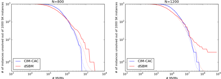
## Chart: Solver Performance Comparison
### Overview
The image presents two line charts comparing the performance of two solvers, CIM-CAC and dSBM, on a set of instances. Both charts depict the number of unsolved instances out of 1000 SK instances against the number of MVMs (Movements). The two charts differ in the value of 'N', representing the number of instances, with the left chart showing N=800 and the right chart showing N=1200.
### Components/Axes
* **X-axis:** "# MVMs" (Number of Movements), logarithmic scale from 10<sup>4</sup> to 10<sup>9</sup>.
* **Y-axis:** "# of instances unsolved out of 1000 SK instances", logarithmic scale from 10<sup>0</sup> to 10<sup>3</sup>.
* **Legend (Left Chart, bottom-right):**
* Blue Line: CIM-CAC
* Red Line: dSBM
* **Legend (Right Chart, bottom-right):**
* Blue Line: CIM-CAC
* Red Line: dSBM
* **Title (Left Chart, top-center):** N=800
* **Title (Right Chart, top-center):** N=1200
### Detailed Analysis or Content Details
**Left Chart (N=800):**
* **CIM-CAC (Blue Line):** The line starts at approximately 1000 unsolved instances at 10<sup>4</sup> MVMs. It gradually decreases, remaining relatively flat until approximately 5 x 10<sup>5</sup> MVMs, where it begins to decline more rapidly. Around 2 x 10<sup>7</sup> MVMs, the line drops sharply to approximately 10 unsolved instances. There is a slight increase and then decrease around 8 x 10<sup>7</sup> MVMs, ending at approximately 5 unsolved instances at 10<sup>9</sup> MVMs.
* **dSBM (Red Line):** The line begins at approximately 1000 unsolved instances at 10<sup>4</sup> MVMs. It decreases more slowly than CIM-CAC initially. Around 3 x 10<sup>6</sup> MVMs, the line begins to decline more rapidly. Around 1 x 10<sup>7</sup> MVMs, the line drops sharply to approximately 20 unsolved instances. It continues to decrease, ending at approximately 2 unsolved instances at 10<sup>9</sup> MVMs.
**Right Chart (N=1200):**
* **CIM-CAC (Blue Line):** The line starts at approximately 1000 unsolved instances at 10<sup>4</sup> MVMs. It decreases gradually, remaining relatively flat until approximately 4 x 10<sup>5</sup> MVMs, where it begins to decline more rapidly. Around 2 x 10<sup>7</sup> MVMs, the line drops sharply to approximately 10 unsolved instances. It continues to decrease, ending at approximately 2 unsolved instances at 10<sup>9</sup> MVMs.
* **dSBM (Red Line):** The line begins at approximately 1000 unsolved instances at 10<sup>4</sup> MVMs. It decreases more slowly than CIM-CAC initially. Around 3 x 10<sup>6</sup> MVMs, the line begins to decline more rapidly. Around 1 x 10<sup>7</sup> MVMs, the line drops sharply to approximately 20 unsolved instances. It continues to decrease, ending at approximately 2 unsolved instances at 10<sup>9</sup> MVMs.
### Key Observations
* Both solvers show a decreasing number of unsolved instances as the number of MVMs increases.
* For both N=800 and N=1200, dSBM initially outperforms CIM-CAC at lower MVM values, but CIM-CAC eventually surpasses dSBM in performance as the number of MVMs increases.
* The performance gap between the two solvers narrows as the number of MVMs increases.
* The sharp drops in both lines indicate a point where the solvers are able to efficiently solve a large number of instances.
* The slight fluctuations in the CIM-CAC line around 8 x 10<sup>7</sup> MVMs (N=800) might indicate a local optimum or a temporary plateau in the solver's progress.
### Interpretation
The charts demonstrate the performance of two different solvers (CIM-CAC and dSBM) in solving a set of SK instances. The number of MVMs represents the computational effort expended. The goal is to minimize the number of unsolved instances.
The data suggests that while dSBM may be more efficient at lower computational costs (fewer MVMs), CIM-CAC ultimately becomes more effective as more computational resources are allocated. This could be due to CIM-CAC employing a more sophisticated, but computationally intensive, search strategy that pays off in the long run.
The difference in performance between N=800 and N=1200 is relatively small, suggesting that the solvers' relative performance is consistent across different instance sizes. The logarithmic scales on both axes highlight the exponential nature of the problem – a small increase in MVMs can lead to a significant reduction in the number of unsolved instances, especially at higher MVM values. The fluctuations observed in the CIM-CAC line for N=800 could be indicative of the solver getting stuck in local optima, requiring additional MVMs to escape and continue the search.