## Charts: Eigenvalue Spectrum and Effective Dimension
### Overview
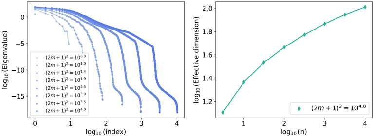
The image presents two charts. The left chart displays the log10 of the Eigenvalues versus the log10 of the index for different values of (2m+1)^2. The right chart shows the log10 of the Effective Dimension versus the log10 of n, also for (2m+1)^2 = 10^0.0.
### Components/Axes
**Left Chart:**
* **X-axis:** log10(index), ranging from approximately 0 to 4.
* **Y-axis:** log10(Eigenvalue), ranging from approximately -15 to 0.
* **Legend:** Located in the top-left corner, listing the following values for (2m+1)^2:
* 10^0.0
* 10^1.4
* 10^1.9
* 10^3.0
* 10^3.5
* 10^4.0
* **Data Series:** Six curves, each representing a different value of (2m+1)^2.
**Right Chart:**
* **X-axis:** log10(n), ranging from approximately 0.5 to 4.
* **Y-axis:** log10(Effective dimension), ranging from approximately 1.1 to 2.0.
* **Legend:** Located in the bottom-right corner, indicating (2m+1)^2 = 10^0.0.
* **Data Series:** A single line representing the relationship between log10(n) and log10(Effective dimension).
### Detailed Analysis or Content Details
**Left Chart:**
* The curves all exhibit a downward trend. The curves start near log10(Eigenvalue) = 0 and decrease to approximately log10(Eigenvalue) = -15.
* (2m+1)^2 = 10^0.0: Starts at approximately log10(Eigenvalue) = 0 and decreases to approximately log10(Eigenvalue) = -15 at log10(index) = 4.
* (2m+1)^2 = 10^1.4: Starts at approximately log10(Eigenvalue) = 0 and decreases to approximately log10(Eigenvalue) = -10 at log10(index) = 4.
* (2m+1)^2 = 10^1.9: Starts at approximately log10(Eigenvalue) = 0 and decreases to approximately log10(Eigenvalue) = -12 at log10(index) = 4.
* (2m+1)^2 = 10^3.0: Starts at approximately log10(Eigenvalue) = 0 and decreases to approximately log10(Eigenvalue) = -14 at log10(index) = 4.
* (2m+1)^2 = 10^3.5: Starts at approximately log10(Eigenvalue) = 0 and decreases to approximately log10(Eigenvalue) = -14 at log10(index) = 4.
* (2m+1)^2 = 10^4.0: Starts at approximately log10(Eigenvalue) = 0 and decreases to approximately log10(Eigenvalue) = -15 at log10(index) = 4.
**Right Chart:**
* The line exhibits an upward trend.
* At log10(n) = 0.5, log10(Effective dimension) is approximately 1.15.
* At log10(n) = 1, log10(Effective dimension) is approximately 1.25.
* At log10(n) = 2, log10(Effective dimension) is approximately 1.5.
* At log10(n) = 3, log10(Effective dimension) is approximately 1.75.
* At log10(n) = 4, log10(Effective dimension) is approximately 1.9.
### Key Observations
* The eigenvalue spectrum (left chart) shows that as (2m+1)^2 increases, the eigenvalues decay more slowly.
* The effective dimension (right chart) increases linearly with log10(n).
* The effective dimension is calculated for the case where (2m+1)^2 = 10^0.0.
### Interpretation
The left chart illustrates the distribution of eigenvalues, which is a key characteristic of a matrix or operator. The different curves represent how the eigenvalue spectrum changes as the parameter (2m+1)^2 is varied. A slower decay in eigenvalues (higher values of (2m+1)^2) suggests that more dimensions are significant in representing the data.
The right chart shows how the effective dimension scales with the size of the input 'n'. The linear relationship indicates that the number of effectively utilized dimensions grows logarithmically with 'n'. This suggests a dimensionality reduction or feature extraction process is at play, where the effective number of dimensions remains relatively small compared to the total number of input features.
The combination of these two charts suggests a relationship between the parameter (2m+1)^2 and the effective dimensionality of the system. Increasing (2m+1)^2 leads to a slower decay of eigenvalues, which in turn implies a higher effective dimension. The right chart provides a quantitative measure of this effective dimension as a function of 'n', for a specific value of (2m+1)^2.