## Line Graph: Learning Rate Schedule
### Overview
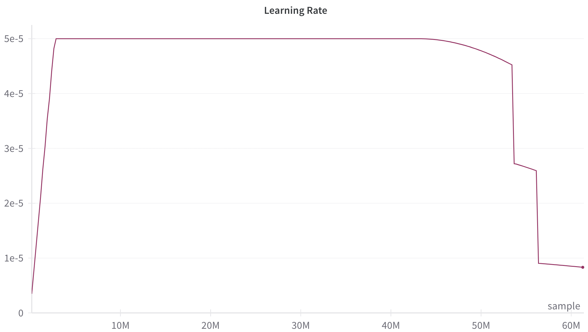
The image displays a line graph titled "Learning Rate," plotting the learning rate value against the number of training samples processed. The graph illustrates a common learning rate schedule used in machine learning model training, characterized by an initial warm-up phase, a prolonged plateau, a gradual decay, and finally, sharp step-wise reductions.
### Components/Axes
* **Title:** "Learning Rate" (centered at the top).
* **Y-Axis (Vertical):** Represents the learning rate value. The axis is labeled with scientific notation markers:
* 0
* 1e-5 (0.00001)
* 2e-5 (0.00002)
* 3e-5 (0.00003)
* 4e-5 (0.00004)
* 5e-5 (0.00005)
* **X-Axis (Horizontal):** Represents the number of training samples. The axis is labeled with markers in millions (M):
* 10M
* 20M
* 30M
* 40M
* 50M
* 60M
* The axis title "sample" is positioned at the bottom-right corner.
* **Data Series:** A single line, colored dark magenta/burgundy, traces the learning rate value across the sample count. There is no separate legend, as only one data series is present.
### Detailed Analysis
The learning rate schedule follows a distinct, multi-phase pattern:
1. **Warm-up Phase (Approx. 0 to 2M samples):** The line begins at or near 0 and rises almost vertically to its maximum value of 5e-5. This steep, near-instantaneous ascent suggests a very short warm-up period.
2. **Plateau Phase (Approx. 2M to 45M samples):** The learning rate remains constant at its peak value of **5e-5**. This forms a long, flat plateau spanning the majority of the training process shown.
3. **Gradual Decay Phase (Approx. 45M to 53M samples):** Starting around the 45M sample mark, the line begins a smooth, concave-downward curve. It decays from 5e-5 to approximately **4.5e-5** by the 53M sample point.
4. **First Step Decay (At ~53M samples):** There is a sharp, vertical drop in the learning rate. The value falls from ~4.5e-5 to approximately **2.8e-5**.
5. **Short Plateau (Approx. 53M to 56M samples):** The learning rate holds steady at ~2.8e-5 for a brief period of about 3 million samples.
6. **Second Step Decay (At ~56M samples):** Another sharp, vertical drop occurs. The learning rate falls from ~2.8e-5 to approximately **0.9e-5**.
7. **Final Phase (56M to 60M+ samples):** The line continues at this lower level, showing a very slight downward trend, ending at a value just below **0.9e-5** at the 60M sample mark.
### Key Observations
* **Dominant Plateau:** Over 70% of the displayed training duration (from ~2M to ~45M samples) occurs at the maximum learning rate.
* **Hybrid Schedule:** The schedule combines a continuous cosine-like decay (from 45M to 53M) with discrete step decays (at 53M and 56M).
* **Aggressive Final Reduction:** The final learning rate is less than 20% of the peak value, indicating a significant fine-tuning phase at the end of training.
* **Noisy Endpoint:** The line at the far right (60M) shows a slight downward jitter, which could be an artifact of the plotting or represent minor fluctuations.
### Interpretation
This graph depicts a sophisticated learning rate schedule designed to optimize the training of a machine learning model, likely a large neural network.
* **Purpose of Phases:** The initial warm-up stabilizes training early on. The long plateau allows the model to make substantial progress with a high learning rate. The subsequent decay phases (both gradual and step-wise) help the model converge to a finer solution by taking smaller steps as it approaches a potential minimum in the loss landscape.
* **Strategic Design:** The combination of a long plateau followed by decay suggests the trainer expects most learning to happen early, with the later stages dedicated to refinement. The two sharp step drops are likely scheduled at predetermined points (e.g., after a certain number of epochs or when a validation metric plateaus) to force the model into a more precise convergence.
* **Contextual Inference:** Such schedules are common in training large language models or other deep learning systems where balancing training stability, speed, and final performance is critical. The specific sample counts (in tens of millions) imply a large-scale training run. The absence of a loss or accuracy curve means we cannot judge the *effectiveness* of this schedule, only its structure.