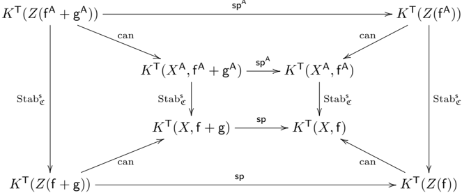
## Commutative Diagram: Algebraic K-Theory/Stabilization Maps
### Overview
The image displays a commutative diagram from advanced mathematics, likely within the fields of algebraic topology, homotopy theory, or algebraic K-theory. It illustrates the relationships and compatibility between several functors or constructions (denoted by `K^T`) applied to different objects (`Z`, `X`) and functions (`f`, `g`), under the operations of stabilization (`Stab^A_e`), specialisation (`sp`, `sp^A`), and canonical maps (`can`). The diagram is structured as a 3x3 grid of nodes connected by horizontal, vertical, and diagonal arrows.
### Components/Axes (Nodes and Arrows)
**Nodes (9 total, arranged in a grid):**
* **Top Row (Left to Right):**
1. `K^T(Z(f^A + g^A))`
2. (Arrow target, no node)
3. `K^T(Z(f^A))`
* **Middle Row (Left to Right):**
1. `K^T(X^A, f^A + g^A)`
2. (Arrow target, no node)
3. `K^T(X^A, f^A)`
* **Bottom Row (Left to Right):**
1. `K^T(Z(f + g))`
2. `K^T(X, f + g)`
3. `K^T(X, f)`
4. `K^T(Z(f))`
**Arrows and Labels:**
* **Horizontal Arrows:**
* Top: `K^T(Z(f^A + g^A))` → `K^T(Z(f^A))` labeled `sp^A`.
* Middle: `K^T(X^A, f^A + g^A)` → `K^T(X^A, f^A)` labeled `sp^A`.
* Middle-Lower: `K^T(X, f + g)` → `K^T(X, f)` labeled `sp`.
* Bottom: `K^T(Z(f + g))` → `K^T(Z(f))` labeled `sp`.
* **Vertical Arrows:**
* Left: `K^T(X^A, f^A + g^A)` → `K^T(X, f + g)` labeled `Stab^A_e`.
* Right: `K^T(X^A, f^A)` → `K^T(X, f)` labeled `Stab^A_e`.
* **Diagonal Arrows (all labeled `can`):**
* Top-Left to Middle-Left: `K^T(Z(f^A + g^A))` → `K^T(X^A, f^A + g^A)`.
* Top-Right to Middle-Right: `K^T(Z(f^A))` → `K^T(X^A, f^A)`.
* Middle-Left to Bottom-Left: `K^T(X^A, f^A + g^A)` → `K^T(Z(f + g))`.
* Middle-Right to Bottom-Right: `K^T(X^A, f^A)` → `K^T(Z(f))`.
### Detailed Analysis
The diagram asserts the commutativity of multiple paths between its nodes. Key relationships include:
1. **Specialisation (`sp^A`, `sp`):** Moving horizontally from left to right corresponds to a map that likely "forgets" or "specialises" the `+ g` (or `+ g^A`) component. This operation is consistent across the `Z` and `X` levels, and between the `A`-superscripted and non-superscripted versions.
2. **Stabilization (`Stab^A_e`):** Moving vertically downward from the `X^A` row to the non-`A` row applies a stabilization map. This map is compatible with the horizontal `sp` maps, forming commutative squares on the left and right sides of the diagram.
3. **Canonical Maps (`can`):** The diagonal arrows represent canonical maps connecting the `Z`-based constructions to the `X`-based ones. These maps are also compatible with both the horizontal `sp` maps and the vertical `Stab^A_e` maps, ensuring the entire diagram commutes.
### Key Observations
* **Symmetry:** The diagram exhibits a high degree of symmetry. The left half (involving `f^A + g^A` and `f + g`) mirrors the right half (involving `f^A` and `f`).
* **Hierarchical Structure:** There is a clear two-level hierarchy: an upper level with objects marked with a superscript `A` (`X^A`, `f^A`, `g^A`) and a lower level without it. The `Stab^A_e` maps connect these levels.
* **Consistency of Operations:** The operations `sp`/`sp^A` and `can` are applied consistently across different contexts (`Z` vs. `X`, with or without `A`), which is the core message of a commutative diagram.
### Interpretation
This diagram is a formal statement of functoriality and compatibility in a sophisticated mathematical theory. It demonstrates that several natural constructions—specializing a function by ignoring an added term (`sp`), stabilizing a structure (`Stab^A_e`), and passing from a `Z`-type object to an `X`-type object (`can`)—all "play well together."
**What it likely means:**
* The `K^T` functor (possibly a variant of topological or algebraic K-theory) preserves these relationships.
* The process of stabilization (`Stab^A_e`) commutes with the specialization map (`sp`). In practical terms, stabilizing a system and then simplifying it yields the same result as simplifying it first and then stabilizing.
* The canonical maps (`can`) provide a bridge between two different but related categories of objects (`Z`-based and `X`-based), and this bridge is consistent with the other operations.
**Why it matters:** Such diagrams are the backbone of proofs in homotopy theory and related fields. They allow mathematicians to track how complex constructions behave under various transformations and ensure that different mathematical pathways lead to consistent results. The commutativity of this specific diagram would be a lemma or proposition used to establish a larger theorem about the properties of the `K^T` functor or the objects `X` and `Z`.
**Language:** The text is entirely in mathematical notation, using Latin letters and standard symbols (`+`, `^`, `_`). No natural language is present.