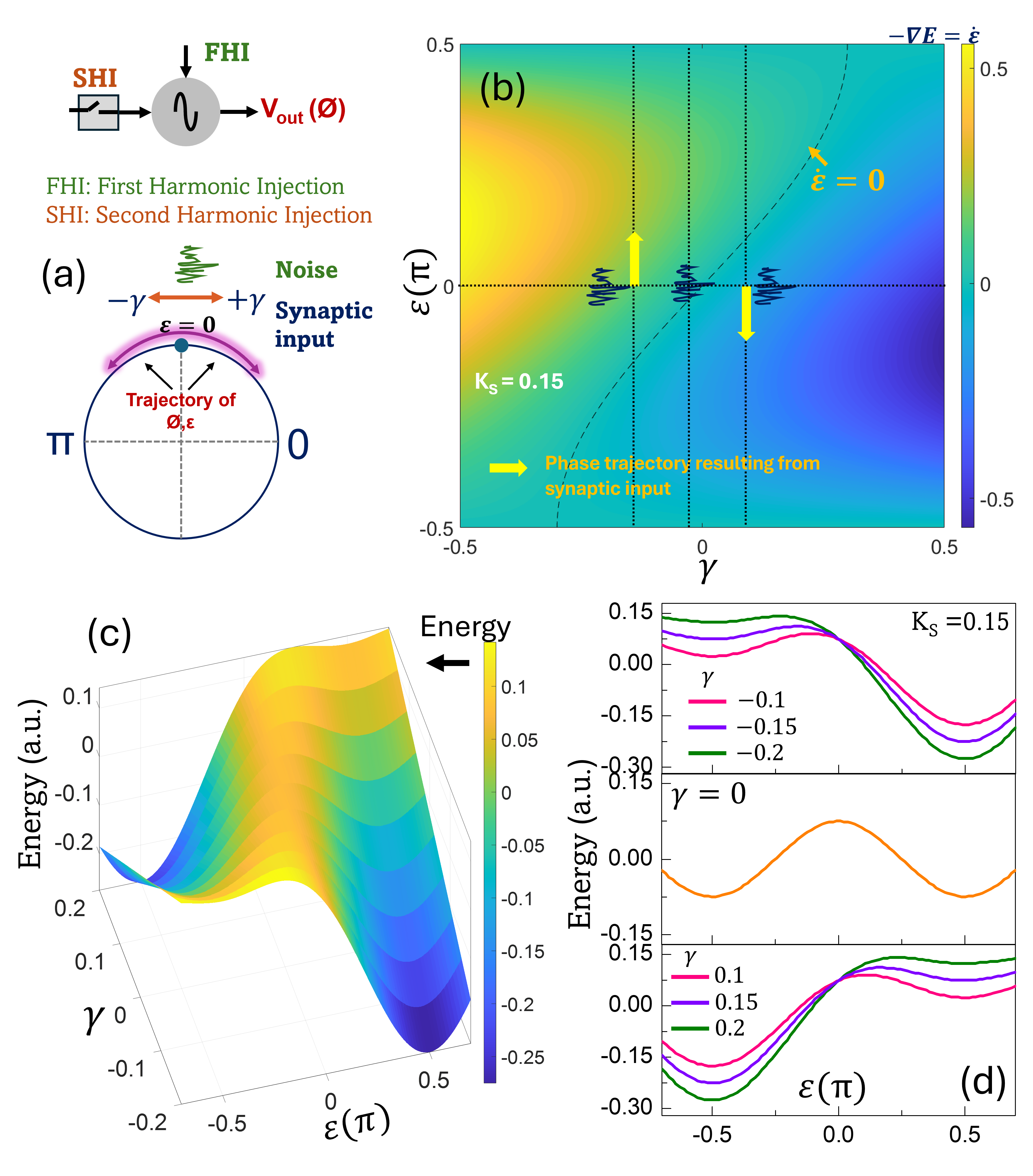
This document provides a technical analysis of the provided image, which illustrates the dynamics of an oscillator system influenced by harmonic injections and synaptic inputs, visualized through phase diagrams, heatmaps, and energy landscapes. ## Diagram: Oscillator Dynamics and Energy Landscapes ### Overview The image is a composite figure containing four distinct panels (labeled a, b, c, and d) and a schematic diagram. It characterizes the behavior of a dynamical system—likely a neural oscillator or similar physical system—subject to First Harmonic Injection (FHI) and Second Harmonic Injection (SHI). The figure explores how parameters $\gamma$ (a bias or control parameter) and $\epsilon$ (a phase-related variable) affect the system's energy landscape and phase trajectory. ### Components/Axes **1. Schematic (Top-Left):** * **Components:** A block diagram showing "SHI" (Second Harmonic Injection) passing through a switch, and "FHI" (First Harmonic Injection) entering a node. The node outputs $V_{out}(\phi)$. * **Text:** * "FHI: First Harmonic Injection" * "SHI: Second Harmonic Injection" **2. Panel (a) - Phase Diagram (Middle-Left):** * **Visual:** A circular representation of phase. * **Labels:** * $\pi$ (left pole), $0$ (right pole), $\epsilon=0$ (top pole). * Arrows labeled $-\gamma$ (pointing left) and $+\gamma$ (pointing right). * Text: "Noise", "Synaptic input", "Trajectory of $\phi, \epsilon$". **3. Panel (b) - Heatmap (Top-Right):** * **Axes:** * X-axis: $\gamma$ (range: -0.5 to 0.5). * Y-axis: $\epsilon$ (range: -0.5 to 0.5). * **Colorbar:** Represents $-\nabla E = \dot{\epsilon}$ (gradient of energy), ranging from -0.5 (dark blue) to 0.5 (yellow). * **Annotations:** * Dashed line labeled "$\dot{\epsilon} = 0$". * Text: "$K_S = 0.15$". * Yellow arrows and wave patterns labeled "Phase trajectory resulting from synaptic input". **4. Panel (c) - 3D Surface Plot (Bottom-Left):** * **Axes:** * X-axis: $\epsilon(\pi)$ (range: -0.5 to 0.5). * Y-axis: $\gamma$ (range: -0.2 to 0.2). * Z-axis: Energy (a.u.) (range: -0.2 to 0.1). * **Colorbar:** "Energy" (range: -0.25 to 0.1). **5. Panel (d) - Line Plots (Bottom-Right):** * **Axes:** * X-axis: $\epsilon(\pi)$ (range: -0.5 to 0.5). * Y-axis: Energy (a.u.) (range: -0.30 to 0.15). * **Legend/Series:** * Top plot ($\gamma < 0$): Pink ($\gamma = -0.1$), Purple ($\gamma = -0.15$), Green ($\gamma = -0.2$). * Middle plot ($\gamma = 0$): Orange ($\gamma = 0$). * Bottom plot ($\gamma > 0$): Pink ($\gamma = 0.1$), Purple ($\gamma = 0.15$), Green ($\gamma = 0.2$). * **Text:** "$K_S = 0.15$". --- ### Detailed Analysis **Panel (a) - Phase Dynamics:** The diagram depicts a circular phase space. The "Trajectory of $\phi, \epsilon$" is shown as a curved arrow along the top arc of the circle. The system is perturbed by "Noise" and "Synaptic input," which shift the trajectory along the $\gamma$ axis. **Panel (b) - Gradient Heatmap:** * **Trend:** The heatmap shows a diagonal transition from yellow (positive $\dot{\epsilon}$) to dark blue (negative $\dot{\epsilon}$). * **Dashed Line:** The line $\dot{\epsilon} = 0$ acts as a separatrix. * **Synaptic Input:** Three vertical dotted lines indicate specific cross-sections where synaptic input causes the phase trajectory to jump or shift, indicated by the yellow arrows. **Panel (c) - 3D Energy Landscape:** * **Trend:** The surface shows a "hill" and "valley" structure. As $\gamma$ increases (moving along the y-axis), the energy landscape deforms. The energy is highest (yellow) at the peak and lowest (blue) in the deep wells. **Panel (d) - Energy vs. Phase:** * **Top Plot ($\gamma < 0$):** The curves show a peak near $\epsilon = 0$ and a dip near $\epsilon = 0.5$. As $\gamma$ becomes more negative (moving from -0.1 to -0.2), the peak height decreases slightly, and the depth of the well increases. * **Middle Plot ($\gamma = 0$):** A single orange curve shows a symmetric oscillation with a peak at $\epsilon \approx 0$ and a minimum at $\epsilon \approx 0.5$. * **Bottom Plot ($\gamma > 0$):** The curves are inverted compared to the top plot. As $\gamma$ increases (0.1 to 0.2), the energy well deepens significantly. --- ### Key Observations * **Symmetry Breaking:** The transition from $\gamma < 0$ to $\gamma > 0$ in panel (d) demonstrates a clear symmetry breaking in the energy landscape. * **Correlation:** The heatmap in (b) is the gradient representation of the energy surface in (c). Where the energy surface is flat (peaks/valleys), the gradient $\dot{\epsilon}$ is zero (the dashed line in b). * **Synaptic Influence:** The synaptic input acts as a forcing function that pushes the system across the energy barriers defined in the landscape. ### Interpretation This figure describes the **bifurcation and control of an oscillator**. * **The System:** The combination of FHI and SHI suggests a system where the phase ($\phi$) is controlled by external harmonic signals. * **The Energy Landscape:** The energy plots (c and d) represent the potential function of the system. The system naturally seeks the lowest energy state (the "wells"). * **The Role of $\gamma$:** $\gamma$ acts as a control parameter that tilts the energy landscape. When $\gamma$ is negative, the system is biased toward one state; when positive, it is biased toward another. * **Synaptic Input:** The synaptic input (visualized in b) provides the energy or "kick" required to move the system's state from one basin of attraction to another across the energy barrier. * **Peircean Investigative Note:** The visual language suggests this is a study in **bistability**. The system can exist in different states, and the "Synaptic input" is the mechanism for switching between these states. The "Noise" mentioned in (a) likely represents stochastic fluctuations that could cause spontaneous switching if the energy barrier is low enough.