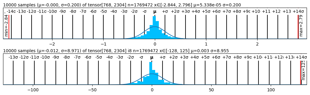
## Histograms: Distribution of Two Tensor Samples ### Overview The image displays two vertically stacked histograms, each visualizing the distribution of 10,000 samples drawn from a tensor with shape [768, 2304]. Both plots include a blue histogram, an overlaid black normal distribution curve, and extensive annotations detailing statistical parameters and standard deviation markers. ### Components/Axes **Top Histogram:** * **Title/Annotation:** `10000 samples (μ=-0.000, σ=0.200) of tensor[768, 2304] n=1769472 x∈[-2.844, 2.796] μ=5.338e-05 σ=0.200` * **X-Axis:** Represents the value range of the samples. Major tick marks are labeled at -2, -1, 0, 1, 2. * **Standard Deviation Markers:** Vertical black lines are placed at intervals of one standard deviation (σ) from the mean (μ). Labels above the axis denote these positions: `-14σ`, `-13σ`, ..., `μ`, `+σ`, `+2σ`, ..., `+14σ`. * **Range Indicators:** A vertical red line on the far left is labeled `min=-2.844`. A vertical red line on the far right is labeled `max=2.796`. * **Legend/Key:** The statistical parameters are embedded in the title annotation. **Bottom Histogram:** * **Title/Annotation:** `10000 samples (μ=-0.012, σ=8.971) of tensor[768, 2304] i8=1769472 x∈[-128, 125] μ=0.003 σ=8.955` * **X-Axis:** Represents the value range of the samples. Major tick marks are labeled at -100, -50, 0, 50, 100. * **Standard Deviation Markers:** Vertical black lines are placed at intervals of one standard deviation (σ) from the mean (μ). Labels above the axis denote these positions: `-13σ`, `-12σ`, ..., `μ`, `+σ`, `+2σ`, ..., `+14σ`. * **Range Indicators:** A vertical red line on the far left is labeled `min=-128`. A vertical red line on the far right is labeled `max=125`. * **Legend/Key:** The statistical parameters are embedded in the title annotation. ### Detailed Analysis **Top Histogram Data & Trend:** * **Distribution Shape:** The histogram shows a very narrow, tall, and symmetric distribution centered at zero. The overlaid normal curve fits the histogram bars closely. * **Statistical Parameters (from title):** * Sample Mean (μ): -0.000 (or 5.338e-05, which is effectively 0.00005338). * Sample Standard Deviation (σ): 0.200. * Data Range (x): [-2.844, 2.796]. * Total Elements (n): 1,769,472. * **Visual Trend:** The data is highly concentrated. The min/max lines at -2.844 and 2.796 correspond to approximately -14.2σ and +14.0σ from the mean, respectively, indicating the extreme tails of the distribution. **Bottom Histogram Data & Trend:** * **Distribution Shape:** The histogram shows a much wider, shorter, and symmetric distribution centered near zero. The overlaid normal curve fits the histogram bars. * **Statistical Parameters (from title):** * Sample Mean (μ): -0.012 (or 0.003 in the second part of the annotation). * Sample Standard Deviation (σ): 8.971 (or 8.955 in the second part of the annotation). * Data Range (x): [-128, 125]. * Total Elements (i8): 1,769,472. * **Visual Trend:** The data is widely spread. The min/max lines at -128 and 125 correspond to approximately -14.3σ and +13.9σ from the mean, respectively. ### Key Observations 1. **Contrasting Spreads:** The most striking observation is the drastic difference in scale between the two distributions. The top distribution has a σ of 0.2, while the bottom has a σ of ~9.0, making the bottom distribution approximately 45 times wider. 2. **Identical Sample Size & Tensor Shape:** Both histograms are derived from tensors of the same shape ([768, 2304]) and contain the same number of total elements (1,769,472), suggesting they may represent different quantizations or transformations of the same underlying data. 3. **Annotation Discrepancy:** The bottom histogram's title contains two slightly different sets of parameters: `(μ=-0.012, σ=8.971)` and later `μ=0.003 σ=8.955`. This could indicate a calculation discrepancy or that the first set refers to the sample and the second to a theoretical distribution. 4. **Extreme Tails:** In both plots, the data range extends to roughly ±14 standard deviations from the mean, which is unusual for a perfect normal distribution and suggests the presence of extreme outliers or a distribution with heavier tails than a Gaussian. ### Interpretation This image likely compares the statistical distributions of two different numerical representations (e.g., different data types like float32 vs. int8, or different scaling factors) of the same underlying dataset or model activations. * **Top Plot (High Precision):** The extremely narrow distribution (σ=0.2) centered at zero is characteristic of normalized data or activations in a neural network, where values are tightly controlled to prevent exploding/vanishing gradients. The near-zero mean is typical after batch normalization. * **Bottom Plot (Low Precision/Quantized):** The wide distribution (σ≈9) spanning from -128 to 125 strongly suggests an 8-bit integer (int8) quantization of the data. The range [-128, 125] is the full dynamic range for signed 8-bit integers. The larger standard deviation indicates the data has been scaled to utilize this full range. * **Relationship:** The pair of plots demonstrates a quantization process. The high-precision, narrow-range values (top) are scaled and possibly shifted to fit into the wider, discrete range of an 8-bit integer format (bottom). The scaling factor would be approximately (range_int8 / range_float) ≈ (250 / 5.6) ≈ 44.6, which aligns with the observed ratio of standard deviations (~9.0 / 0.2 = 45). * **Anomaly:** The presence of data points at ±14σ is statistically highly improbable for a true normal distribution. This indicates the original data, while roughly Gaussian, has "fat tails" or contains outlier values that are preserved through the transformation/quantization process.