## Line Chart: Accuracy vs. Thinking Compute for Different Models
### Overview
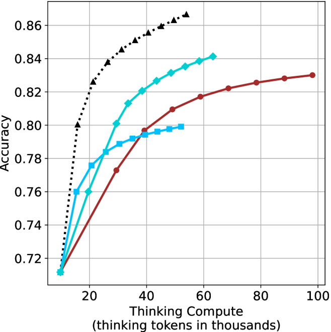
The image is a line chart plotting model accuracy against computational effort, measured in "thinking tokens." It displays four distinct data series, each representing a different model or method, showing how their performance scales with increased compute. The chart demonstrates a clear relationship where accuracy generally increases with more thinking compute, but at different rates and to different saturation points for each series.
### Components/Axes
* **X-Axis (Horizontal):** Labeled "Thinking Compute (thinking tokens in thousands)". The scale runs from 0 to 100, with major tick marks at 20, 40, 60, 80, and 100. The unit is thousands of tokens.
* **Y-Axis (Vertical):** Labeled "Accuracy". The scale runs from 0.72 to 0.86, with major tick marks at 0.72, 0.74, 0.76, 0.78, 0.80, 0.82, 0.84, and 0.86.
* **Data Series (Legend Inferred from Visuals):** There is no explicit legend box. The four series are distinguished by color, line style, and marker shape.
1. **Black, dotted line with upward-pointing triangle markers.**
2. **Cyan (bright blue), solid line with diamond markers.**
3. **Red (dark red/maroon), solid line with circle markers.**
4. **Light blue, solid line with square markers.**
* **Grid:** A light gray grid is present, aligning with the major ticks on both axes.
### Detailed Analysis
**Trend Verification & Data Point Extraction (Approximate Values):**
1. **Black Dotted Line (Triangles):**
* **Trend:** Shows the steepest initial ascent, indicating the highest efficiency in converting compute to accuracy. It begins to plateau at the highest accuracy level among all series.
* **Data Points (Compute k, Accuracy):** (~10, 0.71), (~15, 0.80), (~20, 0.825), (~25, 0.838), (~30, 0.845), (~35, 0.85), (~40, 0.855), (~45, 0.858), (~50, 0.86), (~55, 0.865).
2. **Cyan Solid Line (Diamonds):**
* **Trend:** Shows a strong, steady increase in accuracy that is less steep than the black line initially but continues to climb robustly across the measured range.
* **Data Points (Compute k, Accuracy):** (~10, 0.71), (~15, 0.76), (~20, 0.775), (~25, 0.785), (~30, 0.80), (~35, 0.812), (~40, 0.82), (~45, 0.826), (~50, 0.831), (~55, 0.835), (~60, 0.839), (~65, 0.841).
3. **Red Solid Line (Circles):**
* **Trend:** Exhibits a more gradual, concave-downward curve. It starts lower than the cyan line but surpasses the light blue line and continues to improve steadily, though at a slower rate than the cyan line.
* **Data Points (Compute k, Accuracy):** (~10, 0.71), (~20, 0.74), (~30, 0.772), (~40, 0.797), (~50, 0.809), (~60, 0.817), (~70, 0.822), (~80, 0.826), (~90, 0.828), (~100, 0.83).
4. **Light Blue Solid Line (Squares):**
* **Trend:** Rises quickly at very low compute but then flattens out dramatically, showing strong early saturation. It has the lowest final accuracy of the four series.
* **Data Points (Compute k, Accuracy):** (~10, 0.71), (~15, 0.76), (~20, 0.783), (~25, 0.788), (~30, 0.792), (~35, 0.794), (~40, 0.795), (~45, 0.797), (~50, 0.799).
### Key Observations
* **Performance Hierarchy:** At any given compute level above ~15k tokens, the models maintain a consistent performance order from highest to lowest accuracy: Black > Cyan > Red > Light Blue.
* **Efficiency vs. Saturation:** The black line is the most compute-efficient, reaching ~0.86 accuracy with only ~55k tokens. The light blue line is the least efficient for high accuracy, saturating below 0.80.
* **Convergence at Origin:** All four lines appear to originate from the same point at approximately (10k tokens, 0.71 accuracy), suggesting a common baseline performance with minimal compute.
* **Divergence:** The lines diverge immediately and significantly, highlighting fundamental differences in how each model utilizes additional compute.
### Interpretation
This chart illustrates a core trade-off in AI model design: the relationship between computational investment ("thinking compute") and task performance ("accuracy"). The data suggests:
1. **Diminishing Returns are Model-Dependent:** All models show diminishing returns (the curves flatten), but the point at which returns diminish sharply varies. The light blue model hits this point very early, while the black and cyan models sustain useful gains over a much wider compute range.
2. **Architectural or Methodological Differences:** The starkly different curves imply the models are not just scaled versions of each other. The black-dotted series likely represents a fundamentally more efficient architecture or training paradigm for this specific task, achieving superior accuracy with less computational effort.
3. **Practical Implications:** For applications where compute is cheap or latency is not critical, the cyan or red models might be acceptable. However, for scenarios demanding maximum accuracy per unit of compute (e.g., real-time systems, large-scale deployment), the model represented by the black line is clearly superior. The light blue model appears unsuitable for high-accuracy requirements regardless of compute budget.
4. **The "Thinking" Paradigm:** The axis label "thinking tokens" frames compute as an active reasoning process. The chart validates that for these models, "more thinking" generally leads to better answers, but the quality of the "thinking mechanism" (the model itself) is the primary determinant of final performance.