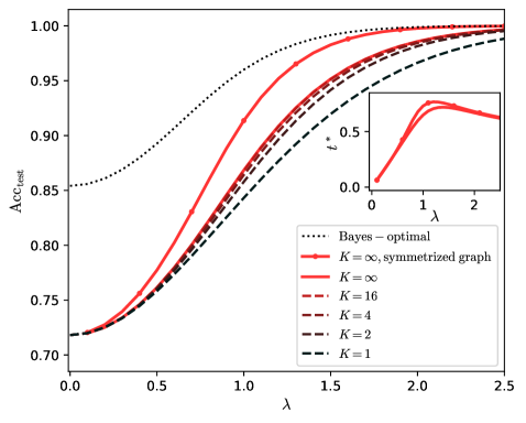
## Line Chart: Accuracy vs. Regularization Parameter (λ) ### Overview The chart compares the test accuracy (Acc_test) of different model configurations against the regularization parameter λ. It includes a main graph and an inset zoomed-in view of the lower λ range. Multiple lines represent different configurations, with the Bayes-optimal performance as a reference. ### Components/Axes - **X-axis (λ)**: Ranges from 0.0 to 2.5 in increments of 0.5. - **Y-axis (Acc_test)**: Ranges from 0.70 to 1.00 in increments of 0.05. - **Legend**: Located in the bottom-right corner, with the following entries: - Dotted black: Bayes-optimal - Solid red: K = ∞, symmetrized graph - Dashed red: K = ∞ - Dashed brown: K = 16 - Dashed maroon: K = 4 - Dashed dark gray: K = 2 - Dashed black: K = 1 - **Inset Graph**: Located in the upper-right corner of the main graph, showing a zoomed-in view of λ ∈ [0, 2] with a secondary y-axis labeled *t*. ### Detailed Analysis 1. **Bayes-optimal (dotted black)**: - Starts at ~0.85 at λ=0 and rises smoothly to ~1.00 by λ=2.5. - Acts as the upper bound for all configurations. 2. **K = ∞, symmetrized graph (solid red)**: - Begins at ~0.72 at λ=0, peaks at ~0.95 near λ=0.5 (inset confirms this), then plateaus near 1.00. - Matches the Bayes-optimal curve closely at higher λ values. 3. **K = ∞ (dashed red)**: - Starts at ~0.70 at λ=0, rises steeply to ~0.95 by λ=1.5, then converges with the Bayes-optimal curve. - Slightly lags behind the symmetrized graph at lower λ values. 4. **K = 16 (dashed brown)**: - Begins at ~0.70 at λ=0, rises to ~0.90 by λ=1.5, then plateaus. - Shows slower convergence compared to higher K values. 5. **K = 4 (dashed maroon)**: - Starts at ~0.70 at λ=0, rises to ~0.85 by λ=1.5, then plateaus. - Demonstrates a trade-off between bias and variance. 6. **K = 2 (dashed dark gray)**: - Begins at ~0.70 at λ=0, rises to ~0.80 by λ=1.5, then plateaus. - Shows limited improvement over K=1. 7. **K = 1 (dashed black)**: - Starts at ~0.70 at λ=0, rises to ~0.75 by λ=1.5, then plateaus. - Minimal improvement over baseline. 8. **Inset Graph**: - Focuses on λ ∈ [0, 2] with a secondary y-axis (*t*). - The red line (K=∞, symmetrized graph) peaks at ~0.95 at λ=0.5, then declines slightly. ### Key Observations - **Bayes-optimal performance** is the theoretical upper limit, approached by all configurations as λ increases. - **Symmetrized graph (K=∞)** achieves the highest accuracy at lower λ values (~0.95 at λ=0.5) compared to non-symmetrized configurations. - **Higher K values** (e.g., K=16, K=4) show better performance than lower K values (e.g., K=2, K=1), indicating that larger neighborhoods improve accuracy. - The **inset graph** highlights a critical region where λ=0.5 maximizes accuracy for the symmetrized graph, suggesting an optimal trade-off between regularization and model complexity. ### Interpretation The chart demonstrates that: 1. **Model complexity (K)** directly impacts accuracy: Higher K values reduce bias, allowing configurations to approach the Bayes-optimal performance. 2. **Symmetrization** enhances performance at lower λ values, suggesting it mitigates overfitting or improves generalization. 3. **Regularization (λ)** balances model complexity and generalization: Too little regularization (low λ) risks overfitting, while excessive regularization (high λ) underfits. 4. The **peak at λ=0.5** in the inset graph implies an optimal regularization strength for the symmetrized graph, balancing bias-variance trade-offs. This analysis aligns with principles of statistical learning theory, where increasing model capacity (via K) and regularization (via λ) jointly optimize performance toward theoretical bounds.