\n
## Scatter Plot: GMM (K=4) on PCA(2) of Residuals
### Overview
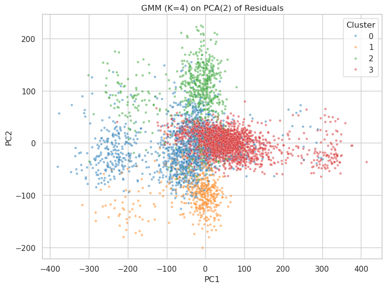
The image is a 2D scatter plot visualizing the results of a Gaussian Mixture Model (GMM) clustering algorithm with 4 clusters (K=4) applied to the first two principal components (PCA(2)) derived from a set of residuals. The plot displays the distribution of data points in a reduced-dimensional space, colored by their assigned cluster.
### Components/Axes
* **Title:** "GMM (K=4) on PCA(2) of Residuals" (centered at the top).
* **X-Axis:** Labeled "PC1". The scale runs from approximately -400 to 400, with major gridlines at intervals of 100.
* **Y-Axis:** Labeled "PC2". The scale runs from approximately -200 to 200, with major gridlines at intervals of 100.
* **Legend:** Located in the top-right corner of the plot area. It is titled "Cluster" and lists four categories with corresponding colored markers:
* Cluster 0: Blue dot
* Cluster 1: Orange dot
* Cluster 2: Green dot
* Cluster 3: Red dot
* **Grid:** A light gray grid is present, aligned with the major ticks on both axes.
### Detailed Analysis
The plot contains four distinct, overlapping clouds of points, each corresponding to a cluster from the GMM.
* **Cluster 0 (Blue):**
* **Spatial Grounding:** Centered in the left-center region of the plot.
* **Trend Verification:** Forms a broad, roughly elliptical cloud. The distribution is densest around PC1 ≈ -100 and PC2 ≈ 0, spreading horizontally from PC1 ≈ -300 to PC1 ≈ 50 and vertically from PC2 ≈ -100 to PC2 ≈ 100.
* **Cluster 1 (Orange):**
* **Spatial Grounding:** Located in the bottom-center region.
* **Trend Verification:** Forms a cloud primarily below the PC2=0 line. It is densest around PC1 ≈ 0 and PC2 ≈ -100, with points spreading from PC1 ≈ -200 to PC1 ≈ 100 and from PC2 ≈ -200 to PC2 ≈ 0.
* **Cluster 2 (Green):**
* **Spatial Grounding:** Located in the top-center region.
* **Trend Verification:** Forms a cloud primarily above the PC2=0 line. It is densest around PC1 ≈ 0 and PC2 ≈ 100, with points spreading from PC1 ≈ -200 to PC1 ≈ 100 and from PC2 ≈ 0 to PC2 ≈ 200.
* **Cluster 3 (Red):**
* **Spatial Grounding:** Located in the right-center region, overlapping significantly with Cluster 0 on its left side.
* **Trend Verification:** Forms a dense, elongated cloud stretching horizontally. It is densest around PC1 ≈ 100 and PC2 ≈ 0, with a long tail extending to the right (positive PC1 direction) up to PC1 ≈ 400. Its vertical spread is roughly from PC2 ≈ -50 to PC2 ≈ 50.
### Key Observations
1. **Cluster Separation and Overlap:** The four clusters show clear separation in the PC2 dimension for Clusters 1 (orange, low PC2) and 2 (green, high PC2). Clusters 0 (blue) and 3 (red) are separated primarily along the PC1 axis but exhibit significant overlap in the central region (PC1 between -50 and 50).
2. **Density and Spread:** Cluster 3 (red) appears to be the most densely packed, especially in its core region. Cluster 0 (blue) has the widest horizontal spread. Clusters 1 and 2 have similar, more compact spreads but are mirrored vertically.
3. **Central Convergence:** All four clusters have a high density of points converging near the origin (PC1=0, PC2=0), indicating a common region in the PCA space where residuals from all groups are similar.
4. **Outliers:** There are sparse outlier points for all clusters, particularly extending from the main clouds. The most notable is the long tail of Cluster 3 extending to high positive PC1 values.
### Interpretation
This plot is a diagnostic tool for understanding the structure of residuals from a statistical or machine learning model. The process involves:
1. **Residual Calculation:** Computing the errors (residuals) of a model's predictions.
2. **Dimensionality Reduction:** Applying Principal Component Analysis (PCA) to the high-dimensional residuals to extract the two most significant directions of variance (PC1 and PC2).
3. **Clustering:** Using a Gaussian Mixture Model to identify 4 distinct subgroups within this 2D residual space.
**What the data suggests:** The presence of four distinct clusters indicates that the model's errors are not random noise but contain systematic patterns. Different subsets of the data (or different underlying conditions) lead to different types of residual behavior. For example:
* **Cluster 2 (Green, high PC2):** Represents a subset where the model consistently makes errors of a specific type captured by high values on the second principal component.
* **Cluster 3 (Red, high PC1):** Represents a subset with errors characterized by high values on the first principal component, which may be the dominant mode of error variance.
* **Overlap between Clusters 0 and 3:** Suggests a continuum or transition zone between two major error regimes.
**Why it matters:** Identifying these clusters allows for deeper model diagnostics. One could investigate what features or data points belong to each cluster to understand *why* the model fails in these specific, patterned ways. This could lead to targeted model improvements, such as collecting more data for a problematic subgroup or engineering features that better capture the patterns currently manifesting as structured residuals. The plot moves beyond a simple aggregate error metric (like MSE) to reveal the *architecture* of the model's failure modes.