## Scatter Plot with Linear Fit: Training Time vs. Number of Spins
### Overview
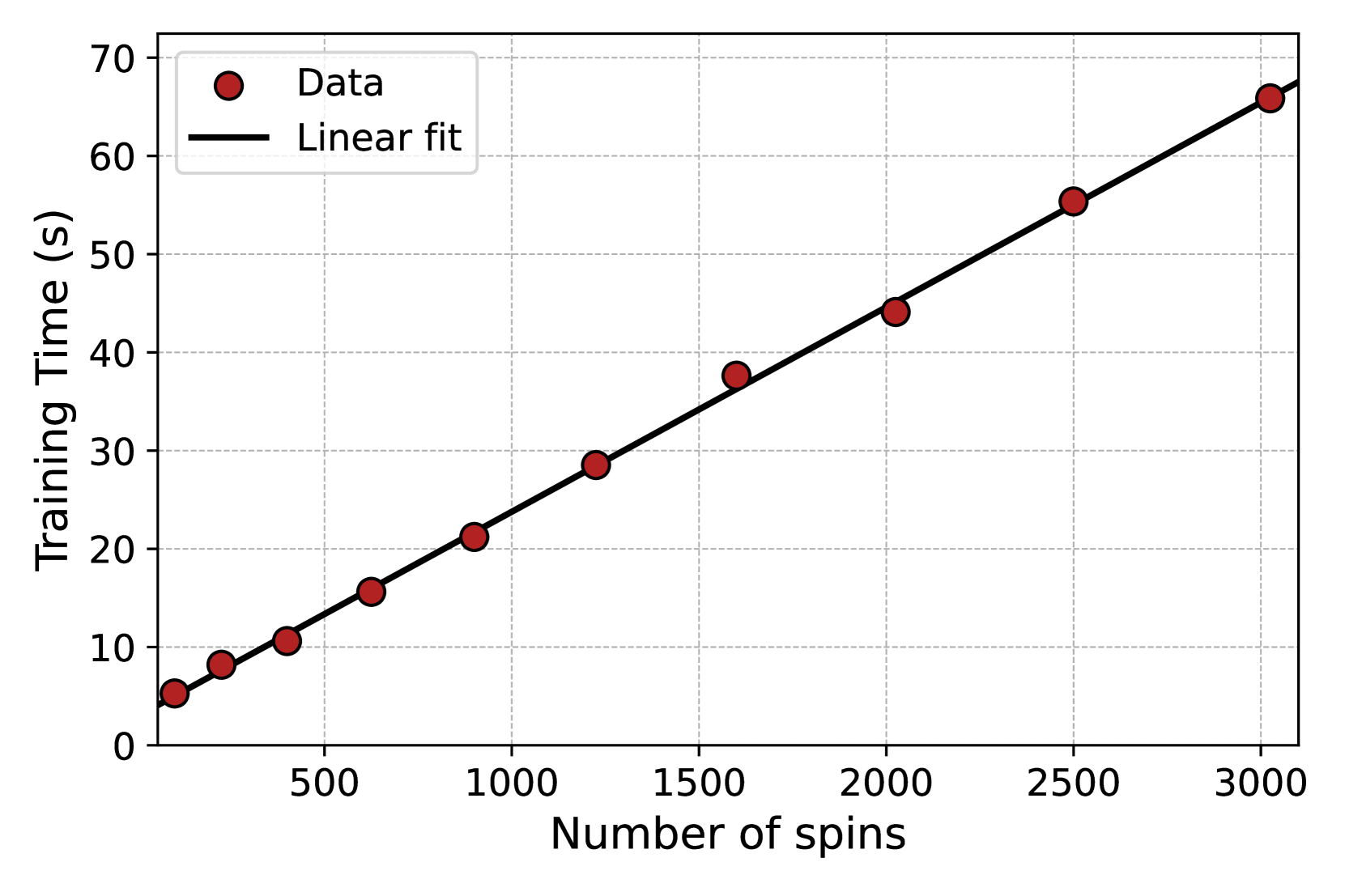
The image is a 2D scatter plot displaying the relationship between the "Number of spins" (independent variable) and "Training Time" in seconds (dependent variable). A set of data points is plotted, and a linear regression line (line of best fit) is drawn through them, indicating a strong positive linear correlation.
### Components/Axes
* **X-Axis (Horizontal):**
* **Label:** "Number of spins"
* **Scale:** Linear scale ranging from 0 to 3000.
* **Major Tick Marks:** 0, 500, 1000, 1500, 2000, 2500, 3000.
* **Y-Axis (Vertical):**
* **Label:** "Training Time (s)"
* **Scale:** Linear scale ranging from 0 to 70.
* **Major Tick Marks:** 0, 10, 20, 30, 40, 50, 60, 70.
* **Legend:** Located in the top-left corner of the plot area.
* **Entry 1:** A red circle symbol labeled "Data".
* **Entry 2:** A solid black line labeled "Linear fit".
* **Grid:** A light gray, dashed grid is present for both major x and y ticks, aiding in value estimation.
### Detailed Analysis
**Data Points (Approximate Coordinates):**
The data consists of 10 red circular points. Their approximate (x, y) coordinates, read from the grid, are:
1. (100, 5)
2. (200, 8)
3. (400, 11)
4. (600, 16)
5. (900, 21)
6. (1200, 29)
7. (1600, 38)
8. (2000, 44)
9. (2500, 55)
10. (3000, 66)
**Linear Fit Line:**
* **Trend:** The black line slopes upward from left to right, confirming a positive linear relationship.
* **Path:** The line passes very close to, or directly through, all plotted data points, indicating an excellent fit.
* **Equation (Estimated):** Based on the endpoints, the line appears to have a y-intercept near 0 and a slope of approximately (66-0)/(3000-0) = 0.022 s/spin. A rough equation is: `Training Time (s) ≈ 0.022 * (Number of spins)`.
### Key Observations
1. **Strong Linear Correlation:** The data points align almost perfectly along a straight line, suggesting the training time scales linearly with the number of spins.
2. **Consistent Spacing:** The data points are not evenly spaced along the x-axis. The sampling density is higher for lower spin counts (e.g., points at 100, 200, 400) and becomes sparser at higher counts (e.g., jumps from 2000 to 2500 to 3000).
3. **Tight Fit:** There is minimal scatter of the data points around the linear fit line. No significant outliers are visible.
### Interpretation
This chart demonstrates a direct, proportional relationship between the computational workload (represented by "Number of spins") and the time required for training. The near-perfect linear fit implies that the underlying algorithm or process has a time complexity of O(n), where n is the number of spins. This is a highly predictable and desirable scaling property, as it means doubling the number of spins will approximately double the training time. The data suggests no evidence of diminishing returns or exponential overhead within the tested range (100 to 3000 spins). For a technical document, this plot serves as strong evidence for the efficient and scalable performance of the system being measured.