## Violin Plot: Predicted Causal Effect (ATE) vs. Dataset Size under Different Scenarios
### Overview
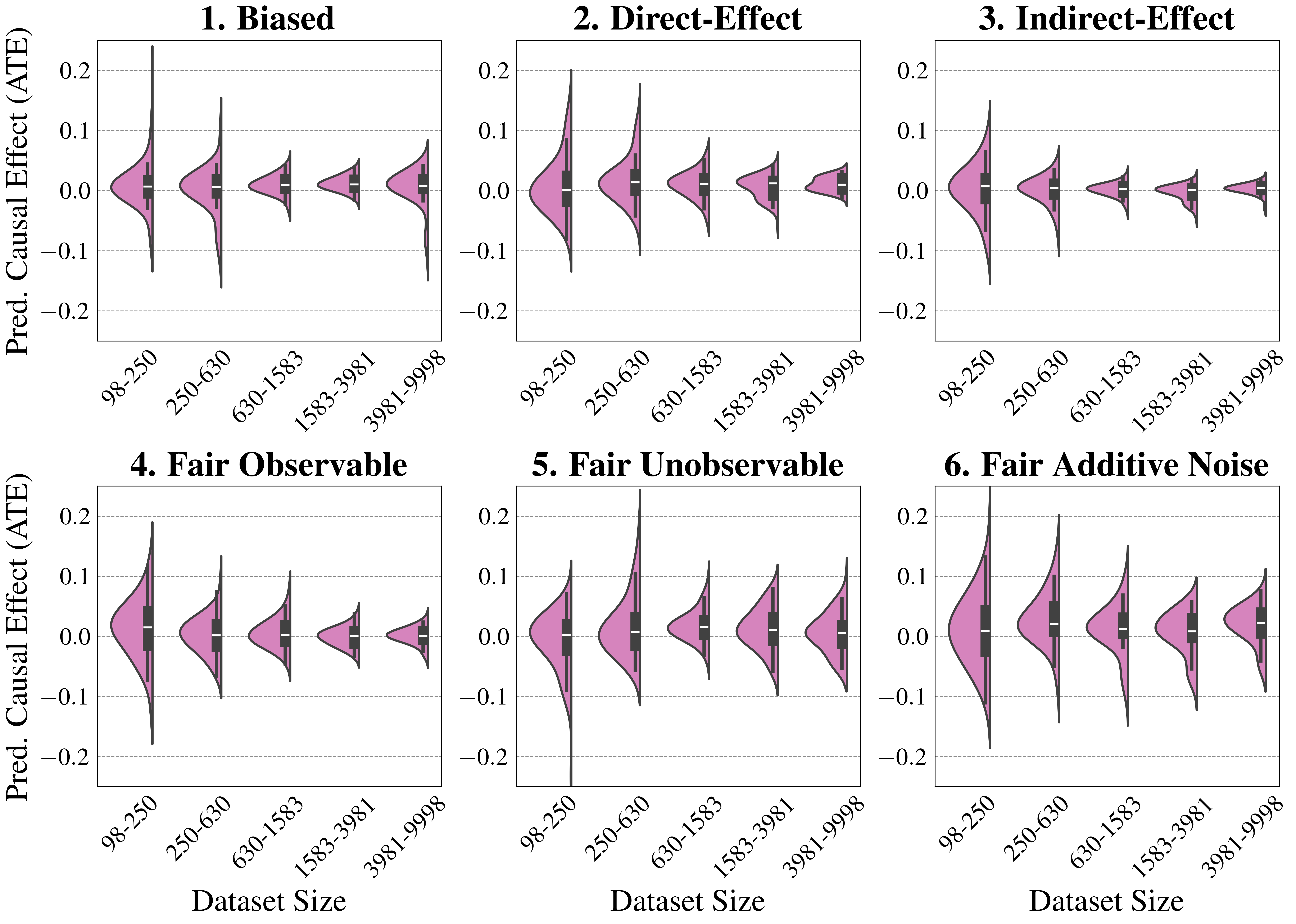
The image presents six violin plots arranged in a 2x3 grid. Each plot visualizes the distribution of predicted causal effects (ATE) for different dataset sizes under varying scenarios: Biased, Direct-Effect, Indirect-Effect, Fair Observable, Fair Unobservable, and Fair Additive Noise. The x-axis represents dataset size, categorized into ranges, while the y-axis represents the predicted causal effect (ATE). The violin plots show the distribution of the predicted causal effect for each dataset size range.
### Components/Axes
* **Y-axis:** "Pred. Causal Effect (ATE)" with a scale from -0.2 to 0.2, marked at -0.2, -0.1, 0.0, 0.1, and 0.2.
* **X-axis:** "Dataset Size" categorized into five ranges: 98-250, 250-630, 630-1583, 1583-3981, and 3981-9998.
* **Violin Plots:** Each violin plot is filled with a light purple color and outlined in black. Each violin plot contains a box plot with a black box and whiskers.
* **Titles:** Each plot has a title indicating the scenario:
1. Biased
2. Direct-Effect
3. Indirect-Effect
4. Fair Observable
5. Fair Unobservable
6. Fair Additive Noise
### Detailed Analysis
**Plot 1: Biased**
* The violin plots show a decreasing spread as the dataset size increases.
* The median (black box) is close to 0 for all dataset sizes.
* The distribution is wider for smaller dataset sizes (98-250 and 250-630) and becomes narrower for larger dataset sizes (1583-3981 and 3981-9998).
**Plot 2: Direct-Effect**
* Similar to the "Biased" scenario, the spread of the violin plots decreases with increasing dataset size.
* The median is close to 0 for all dataset sizes.
* The distribution is wider for smaller dataset sizes and narrower for larger dataset sizes.
**Plot 3: Indirect-Effect**
* The spread of the violin plots decreases with increasing dataset size.
* The median is close to 0 for all dataset sizes.
* The distribution is wider for smaller dataset sizes and narrower for larger dataset sizes.
**Plot 4: Fair Observable**
* The spread of the violin plots decreases with increasing dataset size.
* The median is close to 0 for all dataset sizes.
* The distribution is wider for smaller dataset sizes and narrower for larger dataset sizes.
**Plot 5: Fair Unobservable**
* The spread of the violin plots decreases with increasing dataset size.
* The median is close to 0 for all dataset sizes.
* The distribution is wider for smaller dataset sizes and narrower for larger dataset sizes.
**Plot 6: Fair Additive Noise**
* The spread of the violin plots decreases with increasing dataset size.
* The median is close to 0 for all dataset sizes.
* The distribution is wider for smaller dataset sizes and narrower for larger dataset sizes.
### Key Observations
* In all six scenarios, the spread of the predicted causal effect (ATE) decreases as the dataset size increases. This suggests that larger datasets lead to more precise estimates of the causal effect.
* The medians of the distributions are generally close to 0 across all dataset sizes and scenarios, indicating that the average predicted causal effect is near zero.
* The "Biased" scenario shows a wider distribution for smaller dataset sizes compared to the "Fair" scenarios, suggesting that bias can lead to more variable estimates, especially with limited data.
### Interpretation
The plots demonstrate the impact of dataset size on the precision of predicted causal effects under different scenarios. The consistent trend of decreasing spread with increasing dataset size highlights the importance of having sufficient data for reliable causal inference. The scenarios with "Fair" conditions generally exhibit narrower distributions, suggesting that addressing biases and confounding factors can improve the accuracy and stability of causal effect estimates. The "Biased" scenario shows that even with increasing dataset size, the initial bias can still lead to more variable estimates compared to the "Fair" scenarios. The plots suggest that increasing dataset size can mitigate the impact of noise and unobserved confounders, leading to more precise causal effect estimates.