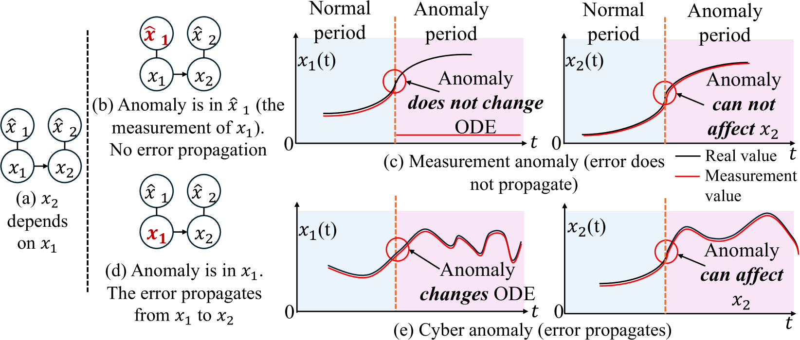
# Technical Document Extraction: Anomaly Propagation in Dynamical Systems This image illustrates the difference between measurement anomalies and cyber (systemic) anomalies within a dynamical system where one variable depends on another. ## 1. System Architecture and Dependency (Left Panel) The left section establishes the causal relationship between variables $x_1$ and $x_2$. ### (a) Dependency Graph * **Components:** Four nodes representing real states ($x_1, x_2$) and their corresponding measurements ($\hat{x}_1, \hat{x}_2$). * **Flow:** A directed arrow points from $x_1$ to $x_2$, indicating that $x_2$ depends on $x_1$. * **Measurement Links:** Vertical lines connect $x_1$ to $\hat{x}_1$ and $x_2$ to $\hat{x}_2$. * **Caption:** "(a) $x_2$ depends on $x_1$" --- ## 2. Scenario 1: Measurement Anomaly (Top Row) This scenario describes an error that occurs only at the sensor/measurement level. ### (b) Logical Diagram * **Anomaly Location:** The node $\hat{x}_1$ is highlighted in red. * **Caption:** "(b) Anomaly is in $\hat{x}_1$ (the measurement of $x_1$). No error propagation" ### (c) Time-Series Analysis The charts plot value ($x(t)$) against time ($t$). A vertical dashed orange line separates the "Normal period" (blue background) from the "Anomaly period" (pink background). **Legend:** * **Black Line:** Real value * **Red Line:** Measurement value #### Chart $x_1(t)$ (Measurement Anomaly) * **Normal Period:** The black and red lines are closely aligned, showing a gradual upward slope. * **Anomaly Period:** * **Trend:** The black line (Real value) continues its smooth upward trajectory. * **Trend:** The red line (Measurement) drops abruptly to a flat constant value near zero. * **Annotation:** A red circle highlights the divergence point. Text states: **"Anomaly *does not change* ODE"**. #### Chart $x_2(t)$ (Measurement Anomaly) * **Normal Period:** Black and red lines are aligned, sloping upward. * **Anomaly Period:** * **Trend:** Both the black and red lines continue to follow the same smooth upward trajectory, unaffected by the fault in $\hat{x}_1$. * **Annotation:** A red circle highlights the transition. Text states: **"Anomaly *can not affect* $x_2$"**. --- ## 3. Scenario 2: Cyber Anomaly (Bottom Row) This scenario describes an anomaly that affects the actual state of the system, leading to error propagation. ### (d) Logical Diagram * **Anomaly Location:** The node $x_1$ is highlighted in red. * **Caption:** "(d) Anomaly is in $x_1$. The error propagates from $x_1$ to $x_2$" ### (e) Time-Series Analysis The charts use the same axes and legend as Scenario 1. #### Chart $x_1(t)$ (Cyber Anomaly) * **Normal Period:** Black and red lines are aligned, sloping upward. * **Anomaly Period:** * **Trend:** Both the black and red lines begin to fluctuate erratically (oscillating up and down). Because the anomaly is in the state $x_1$ itself, the measurement $\hat{x}_1$ tracks the faulty real value. * **Annotation:** A red circle highlights the start of the oscillation. Text states: **"Anomaly *changes* ODE"**. #### Chart $x_2(t)$ (Cyber Anomaly) * **Normal Period:** Black and red lines are aligned, sloping upward. * **Anomaly Period:** * **Trend:** Both the black and red lines exhibit the same erratic, oscillating behavior seen in $x_1$. This demonstrates that the fault in the state of $x_1$ has propagated to the state of $x_2$. * **Annotation:** A red circle highlights the start of the propagated oscillation. Text states: **"Anomaly *can affect* $x_2$"**. --- ## Summary of Key Findings | Feature | Measurement Anomaly (c) | Cyber Anomaly (e) | | :--- | :--- | :--- | | **Primary Fault** | Sensor/Measurement ($\hat{x}_1$) | System State ($x_1$) | | **Effect on ODE** | None (Real value remains smooth) | Changes ODE (Real value becomes erratic) | | **Propagation** | Does not propagate to $x_2$ | Propagates to $x_2$ | | **Measurement Tracking** | Measurement diverges from Real | Measurement follows the faulty Real value |