## Line Charts: Comparison of SA and QA Algorithms
### Overview
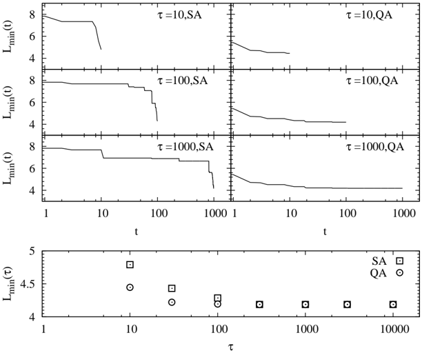
The image presents a series of line charts comparing the performance of two algorithms, Simulated Annealing (SA) and Quantum Annealing (QA), across different time scales (τ = 10, 100, 1000). The charts display the minimum loss, Lmin(t), as a function of time, t, for each algorithm and time scale. A final chart compares Lmin(τ) for SA and QA across a range of τ values.
### Components/Axes
**Top Six Charts (3x2 Grid):**
* **Y-axis:** Lmin(t) - Minimum Loss, ranging from 4 to 8.
* **X-axis:** t - Time, ranging from 1 to 1000, logarithmic scale.
* **Titles:** Each chart has a title indicating the time scale (τ) and the algorithm (SA or QA). The titles are:
* Top-left: τ = 10, SA
* Top-right: τ = 10, QA
* Middle-left: τ = 100, SA
* Middle-right: τ = 100, QA
* Bottom-left: τ = 1000, SA
* Bottom-right: τ = 1000, QA
**Bottom Chart:**
* **Y-axis:** Lmin(τ) - Minimum Loss, ranging from 4 to 5.
* **X-axis:** τ - Time Scale, ranging from 1 to 10000, logarithmic scale.
* **Legend (Top-right):**
* SA: Square symbol
* QA: Circle symbol
### Detailed Analysis
**Top Six Charts (SA):**
* **τ = 10, SA:** Lmin(t) starts at approximately 8, decreases to around 7.5 by t=5, and then drops sharply to approximately 5 by t=10. It remains relatively constant thereafter.
* **τ = 100, SA:** Lmin(t) starts at approximately 8, decreases in steps to approximately 6.5 by t=20, then drops to approximately 5.5 by t=50, and finally drops sharply to approximately 4.5 by t=100. It remains relatively constant thereafter.
* **τ = 1000, SA:** Lmin(t) starts at approximately 8, decreases in steps to approximately 7 by t=20, then drops to approximately 6.5 by t=100, and finally drops sharply to approximately 4 by t=1000. It remains relatively constant thereafter.
**Top Six Charts (QA):**
* **τ = 10, QA:** Lmin(t) starts at approximately 5.5, decreases to approximately 4.5 by t=10, and remains relatively constant thereafter.
* **τ = 100, QA:** Lmin(t) starts at approximately 5, decreases to approximately 4.2 by t=100, and remains relatively constant thereafter.
* **τ = 1000, QA:** Lmin(t) starts at approximately 4.8, decreases to approximately 4.1 by t=1000, and remains relatively constant thereafter.
**Bottom Chart:**
* **SA (Squares):**
* τ = 10: Lmin(τ) ≈ 4.8
* τ = 100: Lmin(τ) ≈ 4.3
* τ = 1000: Lmin(τ) ≈ 4.2
* τ = 10000: Lmin(τ) ≈ 4.2
* **QA (Circles):**
* τ = 10: Lmin(τ) ≈ 4.4
* τ = 100: Lmin(τ) ≈ 4.2
* τ = 1000: Lmin(τ) ≈ 4.1
* τ = 10000: Lmin(τ) ≈ 4.1
### Key Observations
* For SA, the minimum loss Lmin(t) decreases more significantly as τ increases, but the time it takes to reach a stable value also increases.
* For QA, the minimum loss Lmin(t) is generally lower than SA for smaller values of t.
* In the bottom chart, both SA and QA show a decreasing trend in Lmin(τ) as τ increases, but the decrease becomes less pronounced at higher τ values.
* QA consistently achieves a lower minimum loss Lmin(τ) than SA across all τ values in the bottom chart.
### Interpretation
The data suggests that Quantum Annealing (QA) generally outperforms Simulated Annealing (SA) in terms of achieving a lower minimum loss, especially at smaller time scales (t). While SA can eventually reach a comparable minimum loss, it requires a longer time scale (τ) to do so. The bottom chart reinforces this observation, showing that QA consistently achieves a lower Lmin(τ) across a range of τ values. This indicates that QA is more efficient at finding the minimum loss within a given time frame. The diminishing returns observed at higher τ values suggest that there is a limit to how much further the minimum loss can be reduced by increasing the time scale.