## Line Graph: W(τ) vs. τ (Threshold)
### Overview
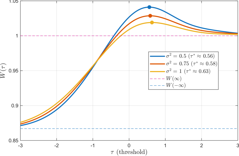
The graph depicts the function \( W(\tau) \) as a function of the threshold parameter \( \tau \), with multiple curves representing different variance values (\( \sigma^2 \)). Key features include:
- A horizontal pink dashed line at \( W = 1 \) (labeled \( W(\infty) \)).
- A horizontal blue dashed line at \( W = 0.85 \) (labeled \( W(-\infty) \)).
- Four solid lines for \( \sigma^2 = 0.5, 0.75, 1 \), and their corresponding peak thresholds (\( \tau^* \approx 0.56, 0.58, 0.63 \)).
### Components/Axes
- **X-axis (τ)**: Labeled "τ (threshold)", ranging from -3 to 3.
- **Y-axis (W(τ))**: Labeled "W(τ)", ranging from 0.85 to 1.05.
- **Legend**: Located in the top-right corner, with:
- Blue line: \( \sigma^2 = 0.5 \) (\( \tau^* \approx 0.56 \)).
- Orange line: \( \sigma^2 = 0.75 \) (\( \tau^* \approx 0.58 \)).
- Yellow line: \( \sigma^2 = 1 \) (\( \tau^* \approx 0.63 \)).
- Pink dashed line: \( W(\infty) \).
- Blue dashed line: \( W(-\infty) \).
### Detailed Analysis
1. **Trends**:
- All curves rise from \( W(-\infty) = 0.85 \) (blue dashed line) as \( \tau \) increases.
- Each curve peaks at a specific \( \tau^* \), then declines toward \( W(\infty) = 1 \) (pink dashed line).
- The peak \( \tau^* \) values increase with \( \sigma^2 \): \( 0.56 \) (blue) < \( 0.58 \) (orange) < \( 0.63 \) (yellow).
- The yellow curve (\( \sigma^2 = 1 \)) has the lowest peak \( \tau^* \), while the blue curve (\( \sigma^2 = 0.5 \)) has the highest.
2. **Data Points**:
- At \( \tau = 0 \), all curves are near \( W = 0.9 \).
- At \( \tau = 1 \), the blue curve (\( \sigma^2 = 0.5 \)) reaches its peak (\( W \approx 1.04 \)).
- At \( \tau = 2 \), all curves converge toward \( W = 1 \).
### Key Observations
- **Peak Behavior**: Higher \( \sigma^2 \) values correspond to lower peak thresholds (\( \tau^* \)), suggesting a trade-off between variance and optimal threshold.
- **Convergence**: All curves asymptotically approach \( W(\infty) = 1 \), indicating a universal upper bound.
- **Asymptotic Bound**: \( W(-\infty) = 0.85 \) acts as a lower bound for all \( \sigma^2 \).
### Interpretation
The graph illustrates how \( W(\tau) \) balances variance (\( \sigma^2 \)) and threshold (\( \tau \)) to achieve a maximum value. The peak \( \tau^* \) represents the optimal threshold for each \( \sigma^2 \), where \( W(\tau) \) is maximized. The convergence to \( W(\infty) = 1 \) implies that increasing \( \tau \) beyond the peak yields diminishing returns, while \( W(-\infty) = 0.85 \) sets a baseline performance limit. This could reflect phenomena like signal detection efficiency, where higher noise (\( \sigma^2 \)) requires lower thresholds to maintain performance, but excessive thresholds risk overshooting the optimal point.