## Chart/Diagram Type: Multi-Panel Figure
### Overview
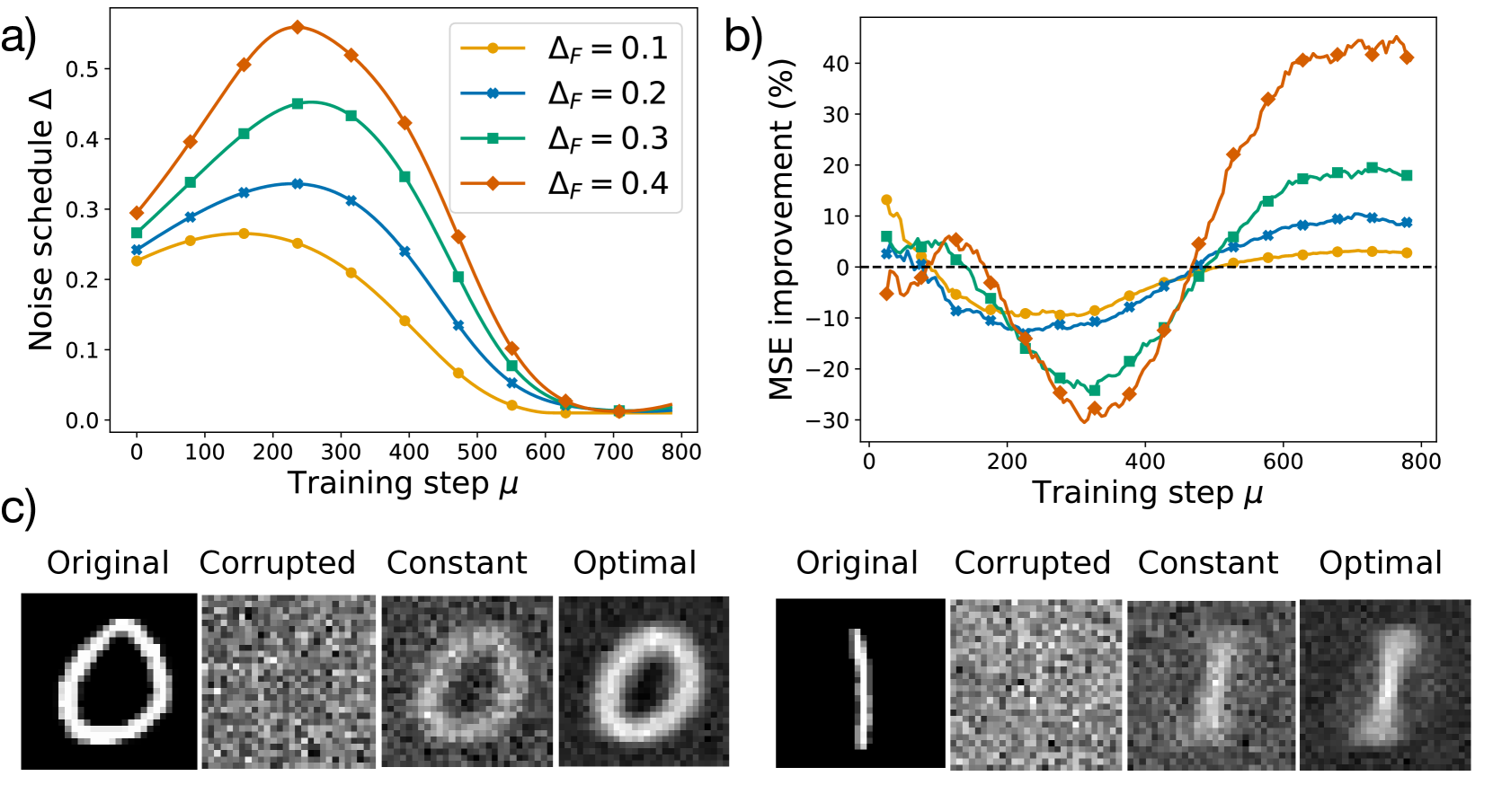
The image consists of three subfigures labeled a), b), and c). Subfigures a) and b) are line plots showing the relationship between training step and noise schedule, and training step and MSE improvement, respectively. Subfigure c) displays example images of digits in original, corrupted, constant, and optimal states.
### Components/Axes
**Subfigure a): Noise Schedule vs. Training Step**
* **Title:** a)
* **X-axis:** Training step μ
* Scale: 0 to 800, with increments of 100.
* **Y-axis:** Noise schedule Δ
* Scale: 0.0 to 0.5, with increments of 0.1.
* **Legend:** Located in the top-right corner of the plot.
* Yellow: ΔF = 0.1
* Blue: ΔF = 0.2
* Green: ΔF = 0.3
* Orange: ΔF = 0.4
**Subfigure b): MSE Improvement vs. Training Step**
* **Title:** b)
* **X-axis:** Training step μ
* Scale: 0 to 800, with increments of 200.
* **Y-axis:** MSE improvement (%)
* Scale: -30 to 40, with increments of 10.
* **Horizontal dashed line:** Represents 0% MSE improvement.
* **Legend:** (Inferred from Subfigure a)
* Yellow: ΔF = 0.1
* Blue: ΔF = 0.2
* Green: ΔF = 0.3
* Orange: ΔF = 0.4
**Subfigure c): Example Images**
* **Labels:**
* Original
* Corrupted
* Constant
* Optimal
* **Images:** Two rows of images, each row containing the four states (Original, Corrupted, Constant, Optimal) of a digit. The top row shows the digit "0", and the bottom row shows the digit "1".
### Detailed Analysis
**Subfigure a): Noise Schedule vs. Training Step**
* **Yellow (ΔF = 0.1):** Starts at approximately 0.23, increases to a peak around 0.27 at a training step of approximately 200, then decreases to approximately 0.02 at a training step of 700-800.
* **Blue (ΔF = 0.2):** Starts at approximately 0.26, increases to a peak around 0.33 at a training step of approximately 200, then decreases to approximately 0.02 at a training step of 700-800.
* **Green (ΔF = 0.3):** Starts at approximately 0.28, increases to a peak around 0.44 at a training step of approximately 250, then decreases to approximately 0.02 at a training step of 700-800.
* **Orange (ΔF = 0.4):** Starts at approximately 0.22, increases to a peak around 0.56 at a training step of approximately 250, then decreases to approximately 0.02 at a training step of 700-800.
**Subfigure b): MSE Improvement vs. Training Step**
* **Yellow (ΔF = 0.1):** Starts at approximately 13%, decreases to a minimum of approximately -12% at a training step of approximately 350, then increases to approximately 3% at a training step of 800.
* **Blue (ΔF = 0.2):** Starts at approximately 4%, decreases to a minimum of approximately -15% at a training step of approximately 350, then increases to approximately 9% at a training step of 800.
* **Green (ΔF = 0.3):** Starts at approximately 7%, decreases to a minimum of approximately -27% at a training step of approximately 350, then increases to approximately 17% at a training step of 800.
* **Orange (ΔF = 0.4):** Starts at approximately -5%, decreases to a minimum of approximately -28% at a training step of approximately 350, then increases to approximately 38% at a training step of 800.
**Subfigure c): Example Images**
* The "Original" images are clear representations of the digits "0" and "1".
* The "Corrupted" images show the digits with added noise, making them difficult to recognize.
* The "Constant" images show the digits after applying a constant noise schedule.
* The "Optimal" images show the digits after applying an optimized noise schedule, resulting in clearer representations compared to the "Constant" images.
### Key Observations
* In subfigure a), as ΔF increases, the peak of the noise schedule also increases. All noise schedules converge to a similar low value at higher training steps.
* In subfigure b), higher ΔF values lead to greater MSE improvement at higher training steps, but also to a greater decrease in MSE improvement at lower training steps.
* In subfigure c), the "Optimal" images are visually better reconstructions of the original digits compared to the "Constant" images.
### Interpretation
The data suggests that the noise schedule (Δ) plays a crucial role in the training process. Higher values of ΔF lead to a more aggressive noise schedule, which initially degrades performance (negative MSE improvement) but ultimately leads to better performance (positive MSE improvement) at later stages of training. The example images in subfigure c) visually confirm that the optimized noise schedule results in better image reconstruction compared to a constant noise schedule. The relationship between ΔF and MSE improvement indicates a trade-off between initial performance and final performance, suggesting that the optimal ΔF value depends on the specific training goals and constraints.