## Neural Network Architectures: Teacher-Student Model
### Overview
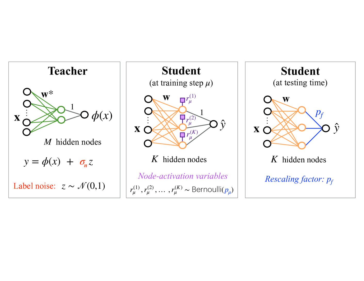
The image presents a diagram illustrating a teacher-student model in machine learning, showcasing the architectures of the teacher network and the student network during training and testing phases. The diagram highlights the flow of information and the key parameters involved in each stage.
### Components/Axes
* **Teacher Network (Left)**:
* Input: x
* Weights: w\*
* Hidden Nodes: M hidden nodes
* Activation Function: φ(x)
* Output: φ(x)
* Label Noise: z ~ N(0,1)
* Equation: y = φ(x) + σ\_n z
* **Student Network (Center)**:
* State: at training step μ
* Input: x
* Weights: w
* Hidden Nodes: K hidden nodes
* Node-activation variables: r\_μ^(1), r\_μ^(2), ..., r\_μ^(K) ~ Bernoulli(p\_μ)
* Output: ŷ
* **Student Network (Right)**:
* State: at testing time
* Input: x
* Weights: w
* Hidden Nodes: K hidden nodes
* Rescaling factor: p\_f
* Output: ŷ
### Detailed Analysis or ### Content Details
**Teacher Network:**
* The input 'x' is fed into the network.
* The network has 'M' hidden nodes.
* The weights connecting the input layer to the hidden layer are denoted as 'w\*'.
* The output of the teacher network is φ(x).
* Label noise 'z' is added to the output, where 'z' follows a normal distribution with mean 0 and standard deviation 1 (N(0,1)).
* The final output 'y' is given by the equation y = φ(x) + σ\_n z, where σ\_n represents the noise level.
* The connections between the input layer and the hidden layer are green.
* The connections between the hidden layer and the output layer are gray.
**Student Network (Training):**
* The input 'x' is fed into the network.
* The network has 'K' hidden nodes.
* The weights connecting the input layer to the hidden layer are denoted as 'w'.
* Node-activation variables r\_μ^(1), r\_μ^(2), ..., r\_μ^(K) follow a Bernoulli distribution with parameter p\_μ.
* The output of the student network is ŷ.
* The connections between the input layer and the hidden layer are orange.
* The connections between the hidden layer and the output layer are gray.
* The node-activation variables are represented by purple squares.
**Student Network (Testing):**
* The input 'x' is fed into the network.
* The network has 'K' hidden nodes.
* The weights connecting the input layer to the hidden layer are denoted as 'w'.
* A rescaling factor 'p\_f' is applied.
* The output of the student network is ŷ.
* The connections between the input layer and the hidden layer are orange.
* The connections between the hidden layer and the output layer are blue.
### Key Observations
* The teacher network has 'M' hidden nodes, while the student network has 'K' hidden nodes.
* The student network's architecture remains the same during training and testing, but the connections to the output node change. During training, the connections are gray, and during testing, the connections are blue.
* The teacher network introduces label noise, while the student network uses node-activation variables during training and a rescaling factor during testing.
### Interpretation
The diagram illustrates a teacher-student learning paradigm, where a student network learns to mimic the behavior of a teacher network. The teacher network provides the target outputs, while the student network adjusts its parameters to minimize the difference between its output and the teacher's output. The use of node-activation variables during training and a rescaling factor during testing suggests that the student network is learning to generalize from noisy data. The teacher network introduces noise to the labels, which forces the student network to learn a more robust representation of the data. The student network uses node-activation variables during training to explore different configurations of the network, and it uses a rescaling factor during testing to adjust the output scale.