## Diagram: Optical Feedback Loop with Measurement
### Overview
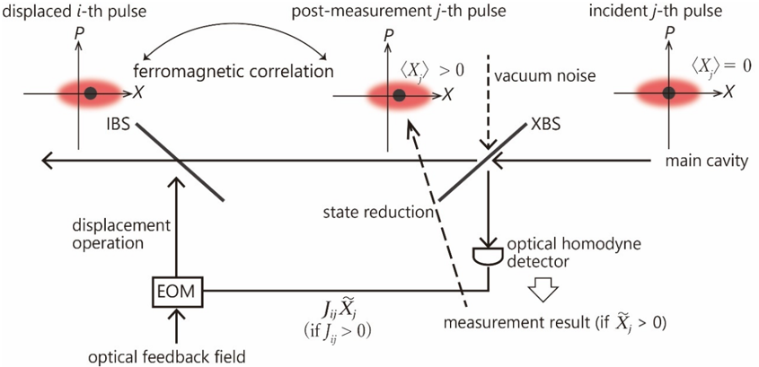
The image is a schematic diagram illustrating an optical feedback loop with measurement, showing the evolution of a light pulse through different stages of interaction and measurement. It depicts the transformation of a displaced i-th pulse, its interaction with a ferromagnetic correlation, the post-measurement j-th pulse, and the incident j-th pulse within a main cavity. The diagram includes optical elements like beam splitters (IBS, XBS), an electro-optic modulator (EOM), and an optical homodyne detector.
### Components/Axes
* **Axes:** Each pulse state is represented on a coordinate plane with axes labeled 'P' (vertical) and 'X' (horizontal).
* **Pulses:**
* "displaced i-th pulse": Located at the top-left.
* "post-measurement j-th pulse": Located at the top-center.
* "incident j-th pulse": Located at the top-right.
* **Optical Elements:**
* "IBS": Imbalanced Beam Splitter.
* "XBS": Another Beam Splitter.
* "EOM": Electro-Optic Modulator.
* "optical homodyne detector": Measures the output signal.
* **Labels:**
* "ferromagnetic correlation": Describes the interaction between the pulses.
* "vacuum noise": Indicates noise affecting the beam.
* "main cavity": Indicates the location of the incident pulse.
* "displacement operation": Describes the operation performed by the EOM.
* "state reduction": Describes the effect of the measurement.
* "optical feedback field": Indicates the feedback signal.
* "measurement result (if X̃j > 0)": Indicates the output of the homodyne detector.
* "Jij X̃j (if Jij > 0)": Describes the feedback signal strength.
* **Expectation Values:**
* "<Xj> > 0": Expectation value of X for the post-measurement pulse.
* "<Xj> = 0": Expectation value of X for the incident pulse.
### Detailed Analysis
1. **Displaced i-th pulse (Top-Left):**
* Axes: P (vertical), X (horizontal).
* A red, roughly circular shape is centered slightly above and to the left of the origin.
* A black dot is located near the center of the red shape.
2. **Post-measurement j-th pulse (Top-Center):**
* Axes: P (vertical), X (horizontal).
* A red, roughly circular shape is centered slightly above and to the right of the origin.
* A black dot is located near the center of the red shape.
* Label: "<Xj> > 0" indicates a positive expectation value for X.
3. **Incident j-th pulse (Top-Right):**
* Axes: P (vertical), X (horizontal).
* A red, roughly circular shape is centered at the origin.
* A black dot is located at the origin.
* Label: "<Xj> = 0" indicates a zero expectation value for X.
4. **Optical Elements and Flow:**
* The "displaced i-th pulse" interacts with the "IBS" (Imbalanced Beam Splitter).
* An arrow labeled "displacement operation" points from the "EOM" (Electro-Optic Modulator) to the "IBS".
* The "post-measurement j-th pulse" interacts with the "XBS".
* A dashed arrow labeled "vacuum noise" points towards the "XBS".
* A dashed arrow labeled "state reduction" connects the "XBS" to the "optical homodyne detector".
* An arrow points from the "optical homodyne detector" to "measurement result (if X̃j > 0)".
* An arrow labeled "optical feedback field" points from the "optical homodyne detector" to the "EOM".
* The "incident j-th pulse" is located in the "main cavity".
* A curved arrow labeled "ferromagnetic correlation" connects the "displaced i-th pulse" to the "post-measurement j-th pulse".
### Key Observations
* The diagram illustrates a closed-loop system where the measurement result influences the input pulse via optical feedback.
* The expectation value of X changes from zero in the incident pulse to positive after measurement.
* The ferromagnetic correlation plays a role in the transformation of the pulse.
### Interpretation
The diagram depicts a quantum feedback loop where the state of a light pulse is manipulated and measured. The "displaced i-th pulse" represents an initial state. The interaction with the "IBS" and the "ferromagnetic correlation" modifies the pulse. The "XBS" and "optical homodyne detector" perform a measurement, resulting in "state reduction". The "optical feedback field" then adjusts the "EOM" to influence the subsequent pulses, closing the feedback loop. The change in the expectation value of X from 0 to >0 indicates a change in the pulse's quadrature amplitude due to the measurement and feedback. The condition "if X̃j > 0" suggests that the feedback is conditional on the measurement outcome. This setup could be used for various quantum control and measurement applications, such as squeezing, entanglement generation, or quantum error correction.