## Chart: CDF of E2E Latency ### Overview The image is a cumulative distribution function (CDF) plot comparing the end-to-end (E2E) latency of SGLang (both non-deterministic and deterministic versions) and LLM-42 at various sparsity levels (2%, 5%, 10%, 20%, 50%, and 100%). The x-axis represents E2E latency in milliseconds (ms), and the y-axis represents the cumulative distribution function (CDF), ranging from 0 to 1. ### Components/Axes * **X-axis:** E2E Latency (ms), with ticks at 0, 20000, 40000, 60000, 80000, and 100000. * **Y-axis:** CDF, with ticks at 0.0, 0.2, 0.4, 0.6, 0.8, and 1.0. * **Legend:** Located on the right side of the plot, it identifies each line by color and label: * Green: SGLang non-deterministic * Red: SGLang deterministic * Blue: LLM-42 @2% * Orange: LLM-42 @5% * Purple: LLM-42 @10% * Brown: LLM-42 @20% * Pink: LLM-42 @50% * Teal: LLM-42 @100% ### Detailed Analysis * **SGLang non-deterministic (Green):** The CDF rises sharply from 0 to 1 between approximately 0 ms and 5000 ms. * **SGLang deterministic (Red):** The CDF rises sharply from 0 to 1 between approximately 0 ms and 15000 ms. * **LLM-42 @2% (Blue):** The CDF rises sharply from 0 to 1 between approximately 0 ms and 10000 ms. * **LLM-42 @5% (Orange):** The CDF rises sharply from 0 to 1 between approximately 0 ms and 12000 ms. * **LLM-42 @10% (Purple):** The CDF rises sharply from 0 to 1 between approximately 0 ms and 20000 ms. * **LLM-42 @20% (Brown):** The CDF rises sharply from 0 to 1 between approximately 0 ms and 20000 ms. * **LLM-42 @50% (Pink):** The CDF rises sharply from 0 to 1 between approximately 0 ms and 40000 ms. * **LLM-42 @100% (Teal):** The CDF rises sharply from 0 to 1 between approximately 0 ms and 40000 ms. ### Key Observations * SGLang non-deterministic has the lowest E2E latency, followed by LLM-42 @2% and LLM-42 @5%. * SGLang deterministic has a higher E2E latency than SGLang non-deterministic. * LLM-42 @10% and LLM-42 @20% have similar E2E latency distributions. * LLM-42 @50% and LLM-42 @100% have the highest E2E latencies among the LLM-42 variants. ### Interpretation The CDF plot illustrates the impact of sparsity on the E2E latency of LLM-42 and compares it to SGLang. Lower sparsity levels (2% and 5%) result in lower latencies, approaching the performance of SGLang. As sparsity increases (10%, 20%, 50%, and 100%), the E2E latency of LLM-42 increases significantly. The deterministic version of SGLang has a higher latency than the non-deterministic version. This suggests that sparsity can be used to trade off model size and performance, but there are diminishing returns as sparsity increases beyond a certain point. The plot highlights the performance differences between different configurations and provides insights into the latency characteristics of these systems.

## Chart: Cumulative Distribution Function of E2E Latency ### Overview The image presents a cumulative distribution function (CDF) plot illustrating the end-to-end (E2E) latency of different language models. The x-axis represents latency in milliseconds (ms), and the y-axis represents the cumulative distribution function (CDF), ranging from 0.0 to 1.0. Several lines are plotted, each representing a different model or configuration. ### Components/Axes * **X-axis Title:** E2E Latency (ms) * **Y-axis Title:** CDF * **Legend:** Located in the top-right corner, listing the following data series: * SGLang non-deterministic (Green) * SGLang deterministic (Red) * LLM-42 @2% (Blue) * LLM-42 @5% (Orange) * LLM-42 @10% (Purple) * LLM-42 @20% (Brown) * LLM-42 @50% (Pink) * LLM-42 @100% (Light Blue) * **Gridlines:** A light gray grid is present to aid in reading values. * **Axis Scale:** X-axis ranges from approximately 0 to 100000 ms. Y-axis ranges from 0.0 to 1.0. ### Detailed Analysis The chart displays the CDF for several models. Here's a breakdown of each line's trend and approximate data points: * **SGLang non-deterministic (Green):** This line starts at approximately CDF 0.0 at E2E Latency 0 ms, rises sharply to CDF 0.8 at approximately 10000 ms, and reaches CDF 1.0 at around 25000 ms. * **SGLang deterministic (Red):** This line starts at approximately CDF 0.0 at E2E Latency 0 ms, rises sharply to CDF 0.8 at approximately 15000 ms, and reaches CDF 1.0 at around 30000 ms. * **LLM-42 @2% (Blue):** This line starts at approximately CDF 0.0 at E2E Latency 0 ms, rises to CDF 0.8 at approximately 30000 ms, and reaches CDF 1.0 at around 60000 ms. * **LLM-42 @5% (Orange):** This line starts at approximately CDF 0.0 at E2E Latency 0 ms, rises to CDF 0.8 at approximately 35000 ms, and reaches CDF 1.0 at around 70000 ms. * **LLM-42 @10% (Purple):** This line starts at approximately CDF 0.0 at E2E Latency 0 ms, rises to CDF 0.8 at approximately 40000 ms, and reaches CDF 1.0 at around 80000 ms. * **LLM-42 @20% (Brown):** This line starts at approximately CDF 0.0 at E2E Latency 0 ms, rises to CDF 0.8 at approximately 45000 ms, and reaches CDF 1.0 at around 90000 ms. * **LLM-42 @50% (Pink):** This line starts at approximately CDF 0.0 at E2E Latency 0 ms, rises to CDF 0.8 at approximately 50000 ms, and reaches CDF 1.0 at around 95000 ms. * **LLM-42 @100% (Light Blue):** This line starts at approximately CDF 0.0 at E2E Latency 0 ms, rises to CDF 0.8 at approximately 55000 ms, and reaches CDF 1.0 at around 100000 ms. ### Key Observations * The SGLang models (both deterministic and non-deterministic) exhibit significantly lower latency compared to the LLM-42 models. * As the percentage increases in the LLM-42 models (@2% to @100%), the latency generally increases. This is evident in the rightward shift of the CDF curves. * The deterministic SGLang model has slightly higher latency than the non-deterministic version. * The LLM-42 models show a relatively consistent increase in latency as the percentage parameter increases. ### Interpretation This chart demonstrates the trade-off between latency and potentially other factors (like accuracy or complexity) in different language models. The SGLang models are faster, suggesting they might be simpler or optimized for speed. The LLM-42 models, while slower, offer a range of configurations (represented by the percentages) that allow for tuning the latency based on application requirements. The CDF plot is useful for understanding the probability of observing a particular latency value for each model. For example, the chart shows that the LLM-42 @2% model has a 50% probability of completing within approximately 30000 ms, while the LLM-42 @100% model has a 50% probability of completing within approximately 55000 ms. The increasing latency with higher percentages in LLM-42 likely indicates increased computational cost associated with more complex processing or larger model sizes.

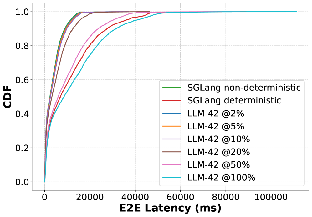
## CDF Chart: End-to-End Latency Comparison ### Overview This image displays a Cumulative Distribution Function (CDF) plot comparing the end-to-end (E2E) latency performance of two systems: "SGLang" (in deterministic and non-deterministic modes) and "LLM-42" at various percentage-based configurations. The chart visualizes the probability (CDF) that a request's latency is less than or equal to a given time value. ### Components/Axes * **Chart Type:** Cumulative Distribution Function (CDF) line chart. * **X-Axis:** Labeled **"E2E Latency (ms)"**. It represents time in milliseconds, with major tick marks at 0, 20000, 40000, 60000, 80000, and 100000. * **Y-Axis:** Labeled **"CDF"**. It represents the cumulative probability, ranging from 0.0 to 1.0, with major tick marks at 0.0, 0.2, 0.4, 0.6, 0.8, and 1.0. * **Legend:** Positioned in the **bottom-right quadrant** of the chart area. It contains 8 entries, each with a colored line sample and a text label: 1. Green line: `SGLang non-deterministic` 2. Red line: `SGLang deterministic` 3. Blue line: `LLM-42 @2%` 4. Orange line: `LLM-42 @5%` 5. Purple line: `LLM-42 @10%` 6. Brown line: `LLM-42 @20%` 7. Pink line: `LLM-42 @50%` 8. Cyan line: `LLM-42 @100%` * **Grid:** A light gray, dashed grid is present for both major X and Y axis ticks. ### Detailed Analysis **Trend Verification & Data Points:** All lines originate at (0 ms, 0.0 CDF) and rise to approach or reach a CDF of 1.0, indicating all measured requests complete within the displayed latency range. 1. **SGLang Lines (Green & Red):** * **Trend:** Both lines exhibit the steepest initial slope, rising very rapidly. * **Data Points:** They cross the 0.8 CDF mark at approximately 5,000-7,000 ms. They reach a CDF of ~0.95 by 20,000 ms and converge to 1.0 shortly after 40,000 ms. The green (non-deterministic) and red (deterministic) lines are nearly coincident, with the red line appearing marginally to the left (slightly lower latency) in the 0.6-0.9 CDF range. 2. **LLM-42 Lines (Blue, Orange, Purple, Brown, Pink, Cyan):** * **General Trend:** These lines show a clear gradient. As the percentage in the label increases, the curve shifts to the right, indicating higher latency for the same cumulative probability. * **LLM-42 @2% (Blue) & @5% (Orange):** These lines closely follow the SGLang lines, being nearly indistinguishable from them in the lower latency region (CDF < 0.8). They are the best-performing among the LLM-42 variants. * **LLM-42 @10% (Purple):** Begins to show a slight rightward shift compared to the @2%/@5% lines, especially noticeable above CDF 0.6. * **LLM-42 @20% (Brown):** Shows a more pronounced rightward shift. It crosses 0.8 CDF at approximately 15,000 ms. * **LLM-42 @50% (Pink):** Has a significantly more gradual slope. It crosses 0.8 CDF at approximately 25,000 ms. * **LLM-42 @100% (Cyan):** Exhibits the most gradual slope and highest latency. It crosses 0.8 CDF at approximately 35,000 ms and does not reach a CDF of 1.0 until near the 100,000 ms mark. ### Key Observations 1. **Performance Hierarchy:** The systems can be grouped by performance: SGLang (both modes) and LLM-42 @2%/@5% form a high-performance cluster. Latency increases progressively for LLM-42 @10%, @20%, @50%, and @100%. 2. **SGLang Deterministic vs. Non-deterministic:** The performance difference between these two modes is minimal, with the deterministic mode showing a very slight advantage. 3. **LLM-42 Parameter Impact:** There is a direct, monotonic relationship between the percentage parameter in the LLM-42 label and end-to-end latency. Higher percentages result in worse (higher) latency across the entire distribution. 4. **Tail Latency:** The "tail" of the distribution (CDF > 0.9) shows the most dramatic differences. For example, to serve 95% of requests (CDF=0.95), SGLang requires ~20,000 ms, while LLM-42 @100% requires nearly 60,000 ms. ### Interpretation This chart demonstrates a clear performance trade-off in the LLM-42 system. The percentage value (e.g., @2%, @100%) likely represents a configuration parameter that trades off latency for another resource or quality metric (such as computational cost, memory usage, or output quality/fidelity). The data suggests: * **SGLang** is optimized for low latency, achieving very fast response times for the vast majority of requests. * **LLM-42** offers a tunable parameter. At low settings (@2%, @5%), it can match SGLang's latency performance. However, increasing this parameter to presumably gain benefits in another dimension (unshown in this chart) comes at a significant and predictable cost to response time. * The **Peircean insight** is that the chart doesn't just show "which is faster," but reveals the *cost function* of the LLM-42 system. The consistent, graded spacing between the LLM-42 curves indicates a well-behaved, predictable relationship between the configuration parameter and its latency impact. This allows a user to make an informed engineering trade-off: selecting the highest LLM-42 percentage that still meets their application's latency budget. The near-overlap of SGLang with LLM-42 @2%/@5% suggests that for latency-critical applications, SGLang or LLM-42 at minimal settings are the viable choices.

## CDF Plot: Latency Distribution Comparison ### Overview The chart compares cumulative distribution functions (CDFs) of end-to-end (E2E) latency for two systems: SGLang (non-deterministic and deterministic variants) and LLM-42 at various percentiles (2%, 5%, 10%, 20%, 50%, 100%). The x-axis represents latency in milliseconds (ms), and the y-axis represents the CDF value (0.0 to 1.0). ### Components/Axes - **X-axis**: E2E Latency (ms), ranging from 0 to 100,000 ms with grid lines at 20,000 ms intervals. - **Y-axis**: CDF (0.0 to 1.0), marked in 0.2 increments. - **Legend**: Positioned in the top-right corner, with color-coded labels: - Green: SGLang non-deterministic - Red: SGLang deterministic - Blue: LLM-42 @2% - Orange: LLM-42 @5% - Purple: LLM-42 @10% - Brown: LLM-42 @20% - Pink: LLM-42 @50% - Cyan: LLM-42 @100% ### Detailed Analysis 1. **SGLang non-deterministic (green)**: - Starts at (0, 0) and rises sharply. - Reaches CDF=1.0 at ~20,000 ms. - Smooth, steep curve with minimal variance. 2. **SGLang deterministic (red)**: - Similar shape to non-deterministic but slightly delayed. - Reaches CDF=1.0 at ~30,000 ms. - Overlaps with LLM-42 @10% (purple) at ~30,000 ms. 3. **LLM-42 percentiles**: - **@2% (blue)**: Reaches CDF=1.0 at ~20,000 ms (matches SGLang non-deterministic). - **@5% (orange)**: Reaches CDF=1.0 at ~25,000 ms. - **@10% (purple)**: Reaches CDF=1.0 at ~30,000 ms (overlaps SGLang deterministic). - **@20% (brown)**: Reaches CDF=1.0 at ~35,000 ms. - **@50% (pink)**: Reaches CDF=1.0 at ~45,000 ms. - **@100% (cyan)**: Reaches CDF=1.0 at ~60,000 ms. ### Key Observations - **SGLang non-deterministic** achieves the lowest latency, outperforming all LLM-42 percentiles except @2%. - **SGLang deterministic** latency aligns with LLM-42 @10%, suggesting similar performance at the 10th percentile. - **LLM-42 @100%** exhibits the highest latency, reaching 1.0 CDF at ~60,000 ms, indicating significant tail latency. - All LLM-42 percentiles show gradual, less steep curves compared to SGLang, implying broader latency distribution. ### Interpretation The data demonstrates that **SGLang non-deterministic** provides the most consistent and lowest-latency performance, making it ideal for latency-sensitive applications. The deterministic variant of SGLang introduces a ~10,000 ms delay compared to its non-deterministic counterpart, aligning it with LLM-42's 10th percentile performance. LLM-42's percentile-based curves reveal a trade-off between average performance and worst-case scenarios: while its 2nd percentile matches SGLang non-deterministic, its 100th percentile latency is 3x higher. This suggests LLM-42 may prioritize throughput or flexibility at the cost of tail latency, whereas SGLang non-deterministic optimizes for minimal latency across all percentiles. The deterministic SGLang variant appears to balance predictability with moderate latency, suitable for applications requiring controlled execution timing.