TECHNICAL ASSET FINGERPRINT
dd1a2f5128d951c8757a5b21
Click to view fullscreen
Press ESC or click to close
FOUND IN PAPERS
EXPERT: gemini-2.0-flash VERSION 1
RUNTIME: nugit/gemini/gemini-2.0-flash
INTEL_VERIFIED
## Neural Network Architecture and Performance Chart
### Overview
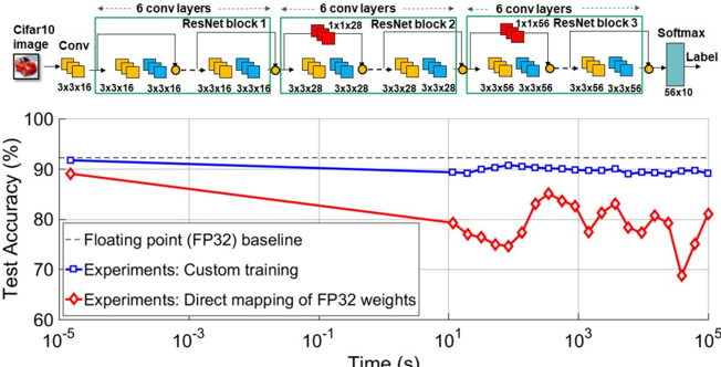
The image presents a diagram of a convolutional neural network (CNN) architecture, followed by a chart comparing the test accuracy of different training methods over time. The CNN architecture consists of convolutional layers and ResNet blocks, while the chart compares the performance of a floating-point baseline, custom training, and direct mapping of FP32 weights.
### Components/Axes
**Top: CNN Architecture Diagram**
* **Header:** "6 conv layers" is repeated above each ResNet block.
* **Input:** "Cifar10 image" followed by "Conv" block.
* The input image is represented by a small image of a red car.
* The "Conv" block has dimensions "3x3x16".
* **ResNet Blocks:** There are three ResNet blocks labeled "ResNet block 1", "ResNet block 2", and "ResNet block 3".
* ResNet block 1: Contains convolutional layers with dimensions "3x3x16".
* ResNet block 2: Contains convolutional layers with dimensions "3x3x28" and a "1x1x28" layer.
* ResNet block 3: Contains convolutional layers with dimensions "3x3x56" and a "1x1x56" layer.
* **Output:** "Softmax" layer with dimensions "56x10" leading to "Label".
* **Connections:** Blocks are connected by arrows indicating the flow of data. Small yellow circles are present at the end of each block.
**Bottom: Test Accuracy Chart**
* **Y-axis:** "Test Accuracy (%)", ranging from 60 to 100. Markers at 70, 80, 90, and 100.
* **X-axis:** "Time (s)" on a logarithmic scale, ranging from 10<sup>-5</sup> to 10<sup>5</sup>. Markers at 10<sup>-5</sup>, 10<sup>-3</sup>, 10<sup>-1</sup>, 10<sup>1</sup>, 10<sup>3</sup>, and 10<sup>5</sup>.
* **Legend (bottom-left):**
* "-- Floating point (FP32) baseline" (dashed black line)
* "Experiments: Custom training" (solid blue line with square markers)
* "Experiments: Direct mapping of FP32 weights" (solid red line with diamond markers)
### Detailed Analysis
**CNN Architecture:**
* The network processes a Cifar10 image through an initial convolutional layer.
* The image then passes through three ResNet blocks, each containing multiple convolutional layers.
* The dimensions of the convolutional layers increase through the network (16 -> 28 -> 56).
* The output of the final ResNet block is fed into a Softmax layer to produce a label.
**Test Accuracy Chart:**
* **Floating point (FP32) baseline (dashed black line):** The baseline accuracy is approximately constant at 92%.
* **Experiments: Custom training (solid blue line with square markers):** The accuracy starts at approximately 90% at 10<sup>-5</sup> seconds, decreases slightly to approximately 89% at 10<sup>1</sup> seconds, and then remains relatively stable around 89-90% until 10<sup>5</sup> seconds.
* **Experiments: Direct mapping of FP32 weights (solid red line with diamond markers):** The accuracy starts at approximately 89% at 10<sup>-5</sup> seconds, decreases to approximately 75% at 10<sup>1</sup> seconds, and then fluctuates between 75% and 85% from 10<sup>1</sup> to 10<sup>5</sup> seconds.
### Key Observations
* The custom training method (blue line) maintains a relatively stable accuracy over time, close to the FP32 baseline.
* The direct mapping of FP32 weights (red line) initially performs similarly to the custom training, but its accuracy degrades significantly over time and exhibits more fluctuation.
* The x-axis is logarithmic, indicating that the performance is being evaluated over a wide range of time scales.
### Interpretation
The data suggests that custom training is a more effective approach than direct mapping of FP32 weights for maintaining accuracy over time. The direct mapping method may suffer from issues related to weight quantization or adaptation, leading to the observed performance degradation and fluctuations. The FP32 baseline provides a benchmark for the maximum achievable accuracy, and the custom training method comes close to achieving this level of performance. The chart highlights the importance of proper training techniques when dealing with different weight representations or hardware constraints.
DECODING INTELLIGENCE...
EXPERT: gemma-3-27b-it-free VERSION 1
RUNTIME: google-free/gemma-3-27b-it
INTEL_VERIFIED
\n
## Chart/Diagram Type: Performance Comparison of Neural Network Training Methods
### Overview
The image presents a comparison of the test accuracy achieved by different training methods for a neural network on the CIFAR-10 dataset, plotted against training time. The top portion of the image shows a diagram of the neural network architecture, while the bottom portion displays a line chart illustrating the performance of three different training approaches: a floating-point (FP32) baseline, custom training, and direct mapping of FP32 weights.
### Components/Axes
* **X-axis:** Time (s), logarithmic scale from 10<sup>-5</sup> to 10<sup>5</sup>.
* **Y-axis:** Test Accuracy (%), ranging from 60% to 100%.
* **Data Series:**
* Floating point (FP32) baseline (dashed red line)
* Experiments: Custom training (blue line with square markers)
* Experiments: Direct mapping of FP32 weights (red line with diamond markers)
* **Neural Network Diagram:** Shows a series of convolutional layers and ResNet blocks.
* Input: CIFAR10 image
* First Layer: Conv (3x3x16)
* ResNet Block 1: 3x3x16 convolutions
* 6 Conv Layers repeated 3 times with increasing filter sizes (1x1x28, 3x3x28, 3x3x56)
* Final Layer: Softmax (56x10)
* Output: Label
* **Legend:** Located in the bottom-left corner, clearly identifying each data series by color and marker type.
### Detailed Analysis or Content Details
The chart displays the test accuracy as a function of training time.
* **Floating Point (FP32) Baseline:** Starts at approximately 91% accuracy at 10<sup>-5</sup> seconds and decreases steadily to around 81% accuracy at 10<sup>5</sup> seconds. The line is relatively smooth.
* **Custom Training:** Begins at approximately 89% accuracy at 10<sup>-5</sup> seconds and remains relatively stable, fluctuating between approximately 88% and 91% accuracy throughout the entire training period (up to 10<sup>5</sup> seconds).
* **Direct Mapping of FP32 Weights:** Starts at approximately 74% accuracy at 10<sup>-5</sup> seconds and increases to around 83% accuracy at 10<sup>2</sup> seconds, then fluctuates significantly between approximately 75% and 85% accuracy for the remainder of the training period.
Specific data points (approximate):
| Time (s) | FP32 Baseline (%) | Custom Training (%) | Direct Mapping (%) |
|---|---|---|---|
| 10<sup>-5</sup> | 91 | 89 | 74 |
| 10<sup>-3</sup> | 90 | 89 | 78 |
| 10<sup>-1</sup> | 88 | 90 | 81 |
| 10<sup>1</sup> | 86 | 89 | 82 |
| 10<sup>2</sup> | 84 | 88 | 83 |
| 10<sup>3</sup> | 82 | 90 | 78 |
| 10<sup>5</sup> | 81 | 91 | 82 |
### Key Observations
* The FP32 baseline exhibits a consistent decrease in accuracy over time, suggesting potential overfitting or diminishing returns.
* Custom training maintains a relatively high and stable accuracy throughout the training process.
* Direct mapping of FP32 weights shows an initial increase in accuracy, followed by significant fluctuations, indicating instability or sensitivity to training parameters.
* Custom training consistently outperforms direct mapping of FP32 weights.
* At the beginning of training, direct mapping starts with significantly lower accuracy than both the baseline and custom training.
### Interpretation
The data suggests that custom training is the most effective method for achieving and maintaining high accuracy on the CIFAR-10 dataset, given the network architecture shown. The FP32 baseline, while starting with high accuracy, degrades over time, potentially due to overfitting. Direct mapping of FP32 weights shows promise with an initial increase in accuracy, but its instability and lower overall performance compared to custom training indicate that it requires further optimization or is not well-suited for this specific network and dataset.
The neural network diagram illustrates a deep convolutional neural network with ResNet blocks, which are known for their ability to mitigate the vanishing gradient problem and enable the training of deeper networks. The architecture appears to be designed for image classification tasks, as evidenced by the final Softmax layer and the CIFAR-10 image input. The diagram provides context for understanding the performance results, as the network's complexity and design choices influence its training dynamics and accuracy. The logarithmic scale on the x-axis highlights the importance of considering training time, especially for computationally intensive tasks like deep learning. The fluctuations in the direct mapping method could be due to the challenges of transferring weights from a higher-precision representation (FP32) to a lower-precision one, potentially leading to quantization errors or instability during training.
DECODING INTELLIGENCE...
EXPERT: healer-alpha-free VERSION 1
RUNTIME: free/openrouter/healer-alpha
INTEL_VERIFIED
## Neural Network Architecture Diagram and Performance Line Graph
### Overview
The image is a composite technical figure containing two primary components: a detailed neural network architecture diagram at the top and a performance line graph at the bottom. The diagram illustrates a ResNet-based convolutional neural network (CNN) designed for image classification on the Cifar10 dataset. The graph below it plots "Test Accuracy (%)" against "Time (s)" on a logarithmic scale, comparing three different training/weight-mapping approaches.
### Components/Axes
#### **Top Component: Neural Network Architecture Diagram**
* **Input:** Labeled "Cifar10 image" with a small icon of a frog.
* **Initial Layer:** A "Conv" layer with a kernel size of "3x3x16".
* **Main Structure:** Three sequential "ResNet block" modules (labeled 1, 2, and 3).
* **ResNet block 1:** Contains "6 conv layers". Internally shows a sequence of layers with kernel sizes: "3x3x16", "3x3x16", "3x3x16", "3x3x16", "3x3x16", "3x3x16". A red block labeled "1x1x56" is shown above, likely representing a shortcut or residual connection.
* **ResNet block 2:** Contains "6 conv layers". Kernel sizes: "3x3x28", "3x3x28", "3x3x28", "3x3x28", "3x3x28", "3x3x28". A red block labeled "1x1x56" is above.
* **ResNet block 3:** Contains "6 conv layers". Kernel sizes: "3x3x56", "3x3x56", "3x3x56", "3x3x56", "3x3x56", "3x3x56". A red block labeled "1x1x56" is above.
* **Output Layers:** Following the blocks is a "Softmax" layer, leading to a final output labeled "Label" with dimensions "56x10".
#### **Bottom Component: Performance Line Graph**
* **Y-Axis:** Labeled "Test Accuracy (%)". Scale ranges from 60 to 100, with major ticks at 60, 70, 80, 90, 100.
* **X-Axis:** Labeled "Time (s)". It is a logarithmic scale with major ticks at 10⁻⁵, 10⁻³, 10⁻¹, 10¹, 10³, 10⁵.
* **Legend:** Located in the bottom-left corner of the graph area. It defines three data series:
1. **Floating point (FP32) baseline:** Represented by a black dashed line.
2. **Experiments: Custom training:** Represented by a blue line with square markers (□).
3. **Experiments: Direct mapping of FP32 weights:** Represented by a red line with diamond markers (◇).
### Detailed Analysis
#### **Graph Data Series and Trends**
1. **Floating point (FP32) baseline (Black Dashed Line):**
* **Trend:** A perfectly horizontal line, indicating constant accuracy over time.
* **Value:** Positioned at approximately 92% accuracy. This serves as the reference benchmark.
2. **Experiments: Custom training (Blue Line with Squares):**
* **Trend:** The line starts near the FP32 baseline at the earliest time point (10⁻⁵ s). It shows a very slight, gradual downward slope as time increases, but remains remarkably stable and high.
* **Key Data Points (Approximate):**
* At 10⁻⁵ s: ~91%
* At 10¹ s: ~90%
* At 10⁵ s: ~89-90%
* **Spatial Grounding:** This blue line is consistently the top-most plotted line (excluding the baseline) across the entire time axis.
3. **Experiments: Direct mapping of FP32 weights (Red Line with Diamonds):**
* **Trend:** This line shows significant degradation and volatility. It starts lower than the custom training line and exhibits a general downward trend with pronounced oscillations (peaks and valleys) as time increases.
* **Key Data Points and Pattern (Approximate):**
* At 10⁻⁵ s: ~89% (starting point).
* It declines to a local minimum of ~75% around 10¹ s.
* It then oscillates, with peaks near 85% (around 10² s) and 82% (around 10⁴ s), and deep valleys near 75% (around 10¹ s) and 68% (around 5x10⁴ s).
* The final point at 10⁵ s is near 81%.
* **Spatial Grounding:** This red line is consistently below the blue "Custom training" line. Its oscillating pattern is visually distinct.
### Key Observations
* **Performance Gap:** There is a clear and persistent performance gap between the "Custom training" method (blue) and the "Direct mapping" method (red). Custom training maintains accuracy within ~2 percentage points of the FP32 baseline, while direct mapping suffers a loss of up to ~24 percentage points at its worst.
* **Stability vs. Instability:** The "Custom training" line is smooth and stable, indicating robust performance over the measured time scale. The "Direct mapping" line is highly unstable, with large fluctuations suggesting sensitivity to the mapping process or training dynamics.
* **Architecture Context:** The network diagram shows a deep architecture (3 blocks * 6 layers = 18 main convolutional layers plus initial and final layers). The increasing channel depth (16 -> 28 -> 56) within the ResNet blocks is a standard design pattern for feature hierarchy learning.
### Interpretation
This figure demonstrates the critical importance of specialized training procedures when deploying quantized or compressed neural network models.
* **The "Direct mapping of FP32 weights"** likely represents a naive approach where a full-precision (FP32) model's weights are directly truncated or rounded to a lower-precision format (e.g., INT8) without any retraining or adaptation. The severe accuracy drop and instability show that this simple discretization destroys the finely-tuned weight relationships, leading to poor and unpredictable model performance.
* **The "Custom training"** approach, in contrast, represents a more sophisticated quantization-aware training (QAT) or post-training optimization scheme. By accounting for the lower precision during the training or fine-tuning process, the model can adapt its weights to maintain high accuracy, nearly matching the original FP32 baseline. The stability of the blue line indicates this method produces a reliably deployable model.
* **The Architecture Diagram** provides necessary context: the performance comparison is being made on a non-trivial, deep ResNet model for image classification. The complexity of the model (multiple residual blocks, increasing depth) makes it more susceptible to performance degradation from naive quantization, underscoring the value of the custom training method shown.
**In summary, the data argues that for practical deployment of efficient, low-precision neural networks, simply copying weights from a high-precision model is insufficient. A dedicated optimization or training process is required to preserve model accuracy and ensure stable performance.**
DECODING INTELLIGENCE...
EXPERT: nemotron-free VERSION 1
RUNTIME: free/nvidia/nemotron-nano-12b-v2-vl:free
INTEL_VERIFIED
## Line Graph: Test Accuracy vs. Time for Neural Network Training
### Overview
The image contains two primary components:
1. A **neural network architecture diagram** (top) depicting a ResNet-based model for CIFAR-10 image classification.
2. A **line graph** (bottom) comparing test accuracy over time for three training methods: FP32 baseline, custom training, and direct mapping of FP32 weights.
---
### Components/Axes
#### Neural Network Diagram
- **Input**: CIFAR-10 image (3x32x32)
- **Layers**:
- 6 convolutional layers (Conv) with 3x3x16 filters
- 3 ResNet blocks (each with 6 convolutional layers):
- Block 1: 3x16x16 → 3x28x28
- Block 2: 3x28x28 → 3x56x56
- Block 3: 3x56x56 → 3x56x56
- Output: Softmax layer (56x10) for label prediction
- **Color Coding**:
- Yellow: Convolutional layers
- Blue: ResNet blocks
- Red: ResNet blocks (highlighted in diagram)
- Gray: Softmax layer
#### Line Graph
- **X-axis**: Time (s) on logarithmic scale (10⁻⁵ to 10⁵)
- **Y-axis**: Test Accuracy (%) from 60% to 100%
- **Legend**:
- Dashed gray: FP32 baseline (90% accuracy)
- Solid blue: Custom training experiments (90% accuracy)
- Red diamonds: Direct mapping of FP32 weights (80–85% accuracy)
---
### Detailed Analysis
#### Neural Network Diagram
- **Flow**:
- Input → 6 Conv layers → ResNet Block 1 → ResNet Block 2 → ResNet Block 3 → Softmax → Label
- **Key Details**:
- ResNet blocks use residual connections (indicated by red arrows in diagram).
- Output dimensions grow from 3x16x16 to 3x56x56 across blocks.
#### Line Graph
1. **FP32 Baseline (Gray Dashed Line)**:
- Constant at ~90% accuracy across all time scales.
2. **Custom Training (Blue Line)**:
- Stable at ~90% accuracy, matching the FP32 baseline.
3. **Direct Mapping of FP32 Weights (Red Diamonds)**:
- Starts at ~85% accuracy, dips below 80% at ~10¹ seconds, then recovers to ~80% by 10³ seconds.
- Exhibits significant volatility compared to other methods.
---
### Key Observations
1. **Accuracy Stability**:
- Custom training and FP32 baseline maintain near-identical accuracy (~90%), suggesting robust performance.
2. **Direct Mapping Limitations**:
- Red line shows a 10% accuracy drop relative to the baseline, with erratic fluctuations.
3. **Time Correlation**:
- Direct mapping’s performance degradation occurs at intermediate time scales (~10¹–10³ seconds).
---
### Interpretation
1. **Model Architecture**:
- The ResNet-based design (with residual connections) likely enables efficient feature extraction, contributing to high accuracy.
2. **Training Method Impact**:
- Direct mapping of FP32 weights introduces instability, possibly due to quantization errors or suboptimal weight initialization.
- Custom training avoids these issues, maintaining performance parity with the FP32 baseline.
3. **Practical Implications**:
- Direct mapping may be unsuitable for production without additional optimization (e.g., fine-tuning).
- The FP32 baseline serves as a critical reference for evaluating quantization trade-offs.
---
### Notable Anomalies
- **Red Line Dip**: The sharp accuracy drop at ~10¹ seconds suggests a potential instability during mid-training phases for direct mapping.
- **Recovery at 10³ Seconds**: Partial recovery implies some adaptation to the training process, but residual performance gaps persist.
DECODING INTELLIGENCE...