# Technical Data Extraction: Conductance (G) vs. $\lambda_I/t$
This document provides a comprehensive extraction of data and trends from the provided scientific plot, which illustrates the conductance ($G$) in units of $e^2/\hbar$ as a function of the dimensionless parameter $\lambda_I/t$.
## 1. Metadata and Global Parameters
The image contains a header indicating the physical parameters held constant for these simulations:
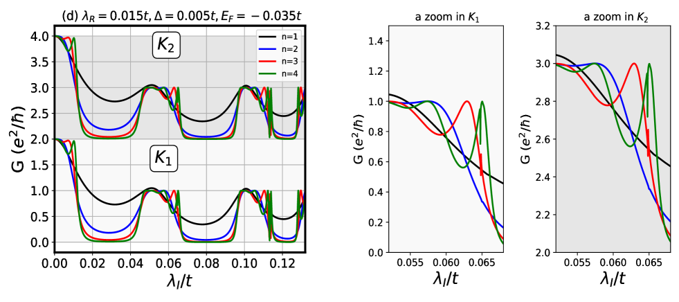
* **Figure Label:** (d)
* **Rashba Coupling ($\lambda_R$):** $0.015t$
* **Exchange/Gap Parameter ($\Delta$):** $0.005t$
* **Fermi Energy ($E_F$):** $-0.035t$
## 2. Main Plot Analysis (Left Panel)
The left panel displays two vertically stacked regions labeled $K_1$ and $K_2$, sharing a common x-axis.
### Axis Definitions
* **X-axis:** $\lambda_I/t$, ranging from $0.00$ to approximately $0.13$.
* **Y-axis:** Conductance $G$ ($e^2/\hbar$).
* **$K_1$ Region (Bottom):** Values range from $0.0$ to $2.0$.
* **$K_2$ Region (Top):** Values range from $2.0$ to $4.0$.
### Legend and Data Series (Spatial Grounding: Top Right of Main Plot)
Four data series are plotted, distinguished by color and the integer parameter $n$:
1. **Black Line ($n=1$):** Shows the smoothest oscillations with the highest minimum conductance values.
2. **Blue Line ($n=2$):** Shows deeper oscillations than $n=1$.
3. **Red Line ($n=3$):** Shows even deeper oscillations and begins to exhibit sharp "dips" or resonances.
4. **Green Line ($n=4$):** Shows the most extreme oscillations, reaching near-zero conductance in the $K_1$ region and near $2.0$ in the $K_2$ region.
### Visual Trends and Observations
* **Periodicity:** The conductance exhibits a periodic "wavy" pattern. Major peaks occur near $\lambda_I/t \approx 0.00, 0.055, 0.105$.
* **Symmetry:** The $K_2$ plot appears to be a vertical translation of the $K_1$ plot (shifted up by $2.0$ units).
* **Resonance Features:** Between $\lambda_I/t = 0.06$ and $0.07$, and again between $0.11$ and $0.12$, the $n=3$ (red) and $n=4$ (green) lines show rapid, sharp fluctuations (Fano-like resonances).
---
## 3. Zoomed-In Analysis (Right Panels)
Two sub-plots provide high-resolution views of the resonance regions for $K_1$ and $K_2$.
### Sub-plot: "a zoom in $K_1$"
* **X-axis:** $\lambda_I/t$ from $0.052$ to $0.068$.
* **Y-axis:** $G$ ($e^2/\hbar$) from $0.0$ to $1.5$.
* **Trend Verification:**
* **Black ($n=1$):** Slopes downward monotonically from $\approx 1.05$ to $\approx 0.45$.
* **Blue ($n=2$):** Slopes downward with a slight inflection, ending near $0.15$.
* **Red ($n=3$):** Oscillates; peaks at $\approx 1.0$ near $0.063$, then drops sharply.
* **Green ($n=4$):** Highly oscillatory; shows a sharp peak reaching $\approx 1.0$ at $\lambda_I/t \approx 0.065$ before a vertical-like drop toward zero.
### Sub-plot: "a zoom in $K_2$"
* **X-axis:** $\lambda_I/t$ from $0.052$ to $0.068$.
* **Y-axis:** $G$ ($e^2/\hbar$) from $2.0$ to $3.2$.
* **Trend Verification:**
* **Black ($n=1$):** Slopes downward from $\approx 3.05$ to $\approx 2.45$.
* **Blue ($n=2$):** Peaks at $\approx 3.0$ near $0.058$, then drops to $\approx 2.15$.
* **Red ($n=3$):** Peaks at $\approx 3.0$ near $0.063$, then drops.
* **Green ($n=4$):** Shows two distinct peaks; the second is very sharp, reaching $\approx 3.0$ at $\lambda_I/t \approx 0.065$.
---
## 4. Data Summary Table (Approximate Values)
| $\lambda_I/t$ (approx) | $G$ ($K_1, n=4$) | $G$ ($K_2, n=4$) | Feature Description |
| :--- | :--- | :--- | :--- |
| 0.00 | 2.0 | 4.0 | Global Maximum |
| 0.03 | 0.0 | 2.0 | Local Minimum (Broad) |
| 0.055 | 1.0 | 3.0 | Local Maximum |
| 0.065 | 1.0 (sharp) | 3.0 (sharp) | Resonance Peak |
| 0.08 | 0.0 | 2.0 | Local Minimum (Broad) |
| 0.105 | 1.0 | 3.0 | Local Maximum |
| 0.115 | 1.0 (sharp) | 3.0 (sharp) | Resonance Peak |
**Note on Language:** All text in the image is in English using standard mathematical notation. No other languages are present.